3. Grouping & Aggregation

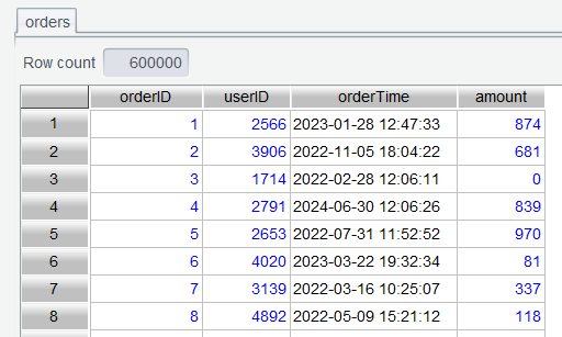
Here are columns of the order table of a supermarket ( orders.csv ):

Column	Description
orderID	Order ID
userID	User ID
orderTime	Order time
amount	Order amount

The table contains 3-year supermarket’s order data from 2022 to 2024.

4.1 Compute sales by year and month

Since we just need the target summary table, there is no need to add a year-month computed column. You can directly use year-month expression as the grouping expression to group orders records.

Step 1: Open orders table:

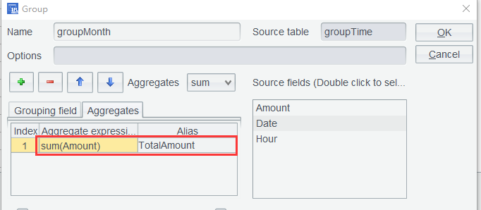
Step 2: Set grouping fields through grouping expression year(orderTime):Year and month(orderTime):Month on orders table:

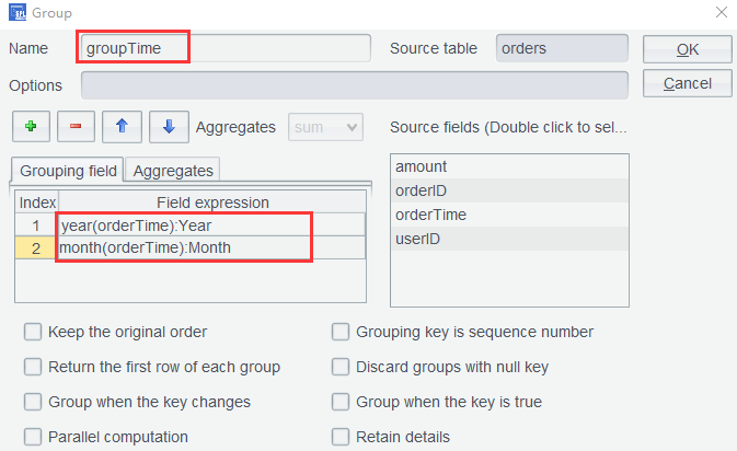
And set aggregate expression to compute sales amount:

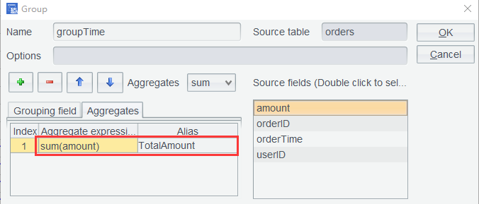
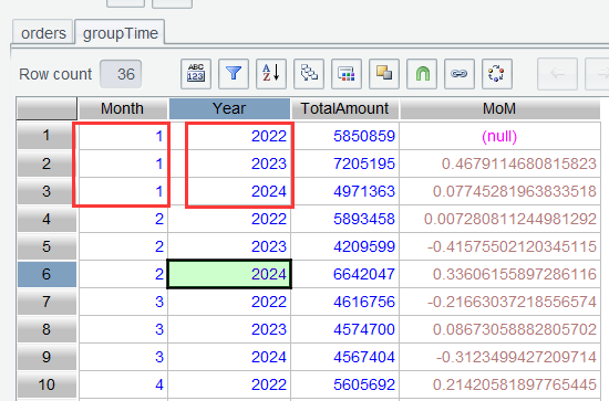
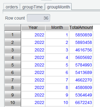
Click OK and get the a table of sales amounts grouped by year and month:

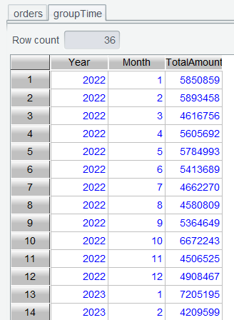
Learning point: month() function is used to get the month to which the specified date belongs. Find its uses HERE.

4.2 Compute sales MoM

The Month-over-Month (MoM) Growth Rate is the rate of change of a certain indicator (such as sales amount, user count, GDP, etc.) between two neighboring time periods (usually month or quarter) . It is used to measure the short-term trend of change.

MoM formula: MoM=(value of the current period− value of the preceding period)/ value of the preceding period

The formula shows that data should be ordered to compute the rate. In Section 4.1, groupTime table was already ordered by year and month, so we can directly compute MoM on the computed column.

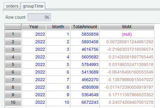
Step 1: Click Computed column for groupTime table and set its expression as (TotalAmount-TotalAmount[-1])/TotalAmount[-1]:

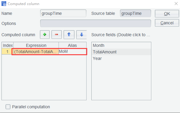
Step 2: Click OK to finish computing the MoM.

4.3 Compute YoY growth rate

The Year-over-Year (YoY) Growth Rate is the rate of change of a certain indicator (such as sales amount, profit, GDP, etc.) between same time periods in different years . It is used to eliminate the seasonal effects to reflect the long-term trend of change.

Formula: YoY=(value of the current period−value of the last year’s same period)/value of the last year’s same period

In Section 3.6, we introduced and explained a method, which groups a data table into multiple details tables, performs computation on each details subtable, and concatenates the result sets. Here we introduce another method. It does not perform the month-based grouping, but it directly compares neighboring rows through a computing expression instead. For convenience of referencing the row of a neighboring year, first put yearly data rows of the same month together.

Step 1: On groupTime table, select header of Month column, click Shift Column Left to move Month column forward to make YoY data view more intuitive:

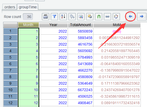
Step 2: Sort groupTime table by Month and Year in ascending order:

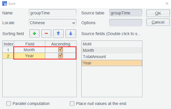
And get a table where rows of neighboring years in the same month are put together:

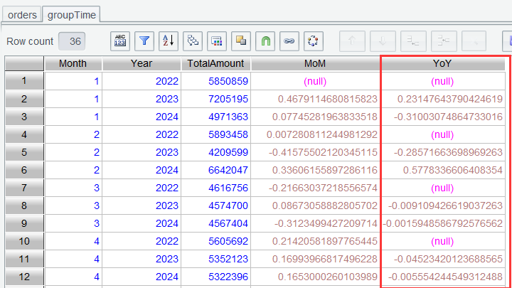
Step 3: Use formula if(Year[-1]==Year-1 && Month[-1]==Month, (TotalAmount-TotalAmount[-1])/TotalAmount[-1], null) to compute YoY growth rate. The formula computes YoY represented by (TotalAmount-TotalAmount[-1])/TotalAmount[-1] when the current pair of neighboring rows belong to the same month and have neighboring years; otherwise, the YoY is null:

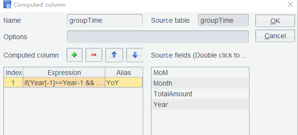
Click OK to get the YoY growth rate:

4.4 Compute 5-day moving average

Moving average is a statistical method used to analyze time series data. It smooths out short-term fluctuations and helps reveal long-term trends by computing the average of data within a specific time window. This method is widely applied in fields such as finance (e.g., stock analysis), economics, meteorology, and quality control.

Formula: MAn=(p1+p2+⋯+pn)/n

Where pn is data of the nth day (such as closing price) and n is the window size (such as 5 days).

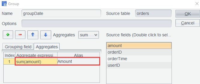
Step 1: On orders table, use expression date(orderTime):Date to remove the time part of the date value and configure grouping by date:

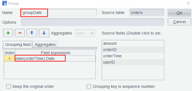
Set aggregate expression to compute sales amount ( Amount ) per day, as the following shows:

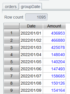
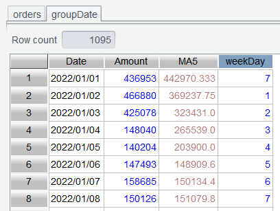
Click OK to get a sales amount table grouped by date:

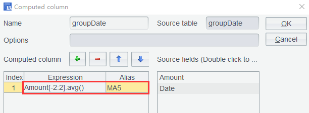
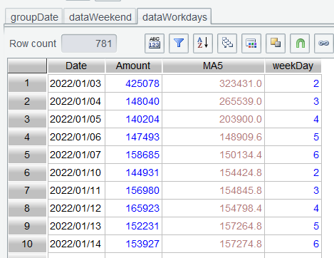
Step 2: Add a Computed Column in groupDate table by setting the expression as Amount[-2:2].avg():

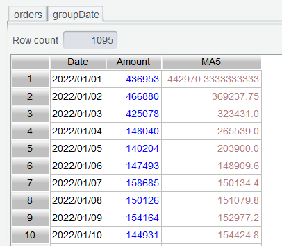
Click OK and get the 5-day moving average:

Learning point: What does Amount[-2:2] mean?
In Section 3.8, we learned that [n] can be used to reference a value at a position relative to the current row. In this section syntax [b:e] defines a reference range from the starting position to the ending position and returns a sequence of values within the range. Amount[-2:2] gets a sequence of values from the current row’s preceding two rows to the next two rows (including the current row).

4.5 Weekdays vs Weekend sales comparison

Implementation approach: After rows are grouped by date, find what day each date is, select rows of Sunday and Saturday and those of weekdays respectively, and compute their respective average sales amount to get the comparison result.

Step 1: Add a Computed Column in groupDate table by setting the expression as day@w(Date):

Click OK to get a table containing number of the day of week:

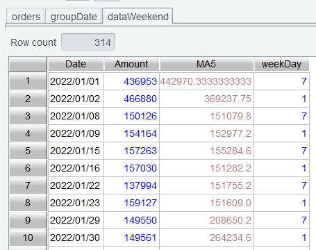
Step 2: Select rows of weekends from table groupDate and perform filtering using expression weekDay==1 || weekDay==7:

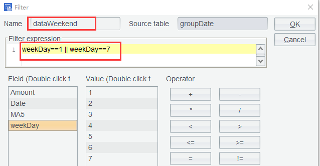
Click OK to get a table of weekend data:

Step 3: Click Set Operations icon on groupDate table:

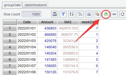
Set target table name, select Difference as the Operator, and select the target table dataWeekend:

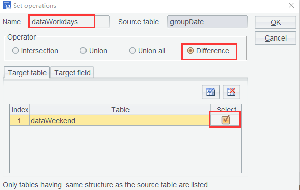
This step of computation finds difference between groupDate and dataWeekend , which are the week data rows obtained by removing weekend data rows from groupDate :

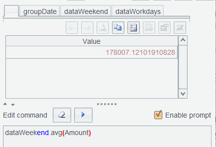
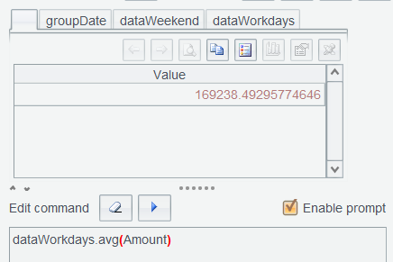
Step 4: In Edit Command Zone, compute dataWeekend.avg(Amount) and dataWorkdays.avg(Amount) respectively:

Learning point : The day@w() function gets which day of the week a given date falls on. It returns 1 for Sunday, 2 for Monday, …, and 7 for Saturday. Find detailed uses HERE.

4.6 Time slot sales contribution

Implementation approach: Group orders table rows by hour, compute hourly average sales amount, and find hourly sales contribution to observe sales peaks and troughs during a day.

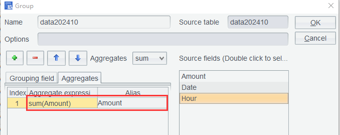
Step 1: Re-open orders table, set grouping expressions date(orderTime):Date and hour(orderTime):Hour in Group window to group rows by the specific time slot for each day:

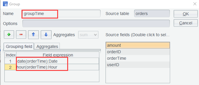
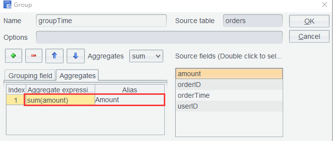
And set aggregate expression sum(amount) to compute total sales:

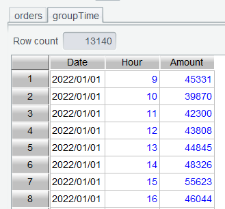
Click OK to get a result table aggregated by hour:

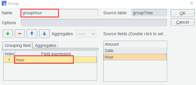
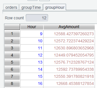
Step 2: Group groupTime table again by Hour field and compute average sales ( AvgAmount ):

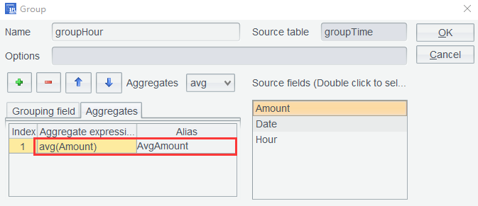
Click OK to get average sales in each time slot:

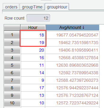
Step 3: Double-click column headers of AvgAmount to sort the table in descending order. Now we can view the sale peaks:

4.7 Sales performance tracking

Set monthly average sales as the monthly sales target, and find daily cumulative sales target achievement for October 2024.

First, compute monthly average sales.

Step 1: Group groupTime again by setting grouping expressions as year(Date):Year and month(Date):Month:

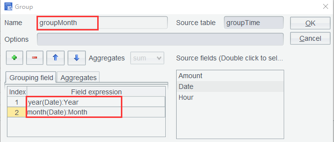
Compute monthly total sales:

Click OK to compute monthly sales amount in each year:

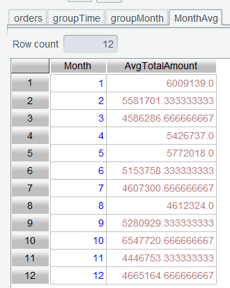
Step 2: roup groupMonth the second time by setting grouping expression as Month:

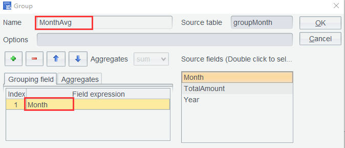
Compute monthly average sales:

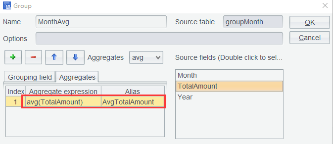
Click OK to compute monthly average sales:

And then daily cumulative sales target achievement for October 2024.

Step 3: Select data rows of October 2024 from groupTime by setting filter expression as year(Date)==2024 && month(Date)==10:

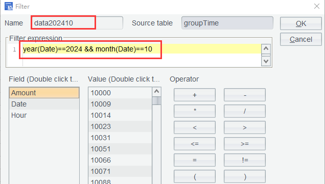
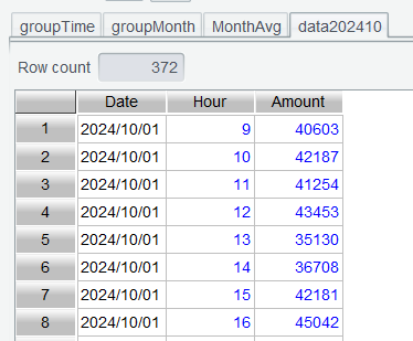
Click OK to get rows of October 2024:

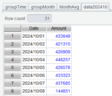
Step 4: Perform aggregation on data202410 by date – again group rows and aggregate by Amount:

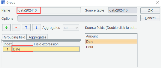
Since the intermediate table grouped by the specified time slot isn’t needed anymore, we still name this grouping result table data202410 and perform sum operation by the time slot:

Click OK and data202410 is aggregated by date:

Step 5: Add a computed column in data202410 to compute the cumulative amount for each date while computing the proportion of the cumulative amount in the average total:

Using expressions:
cum[-1]+Amount
cum/MonthAvg(10).AvgTotalAmount

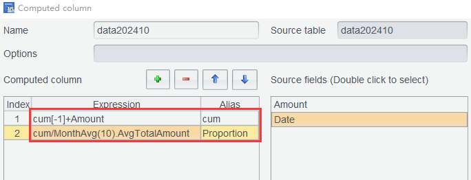
Click OK to compute the cumulative amount and the daily cumulative completion rate:

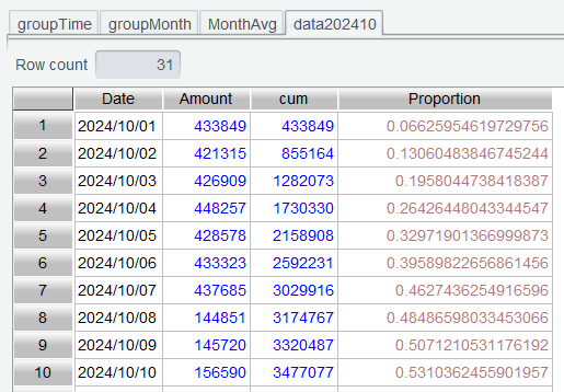
Expression MonthAvg(10).AvgTotalAmount gets the 10^th row from MonthAvg table and then value of its AvgTotalAmount column.

4.8 Purchase cycle analysis

We consider users who make multiple purchases within the same day as purchasing forgotten items or as placing split orders to take advantage of promotions. These are not regarded as repeat purchases. Therefore, we deduplicate such records by date.

Step 1: Open orders table again and deduplicate records by userID and orderTime. Perform grouping settings as follows:

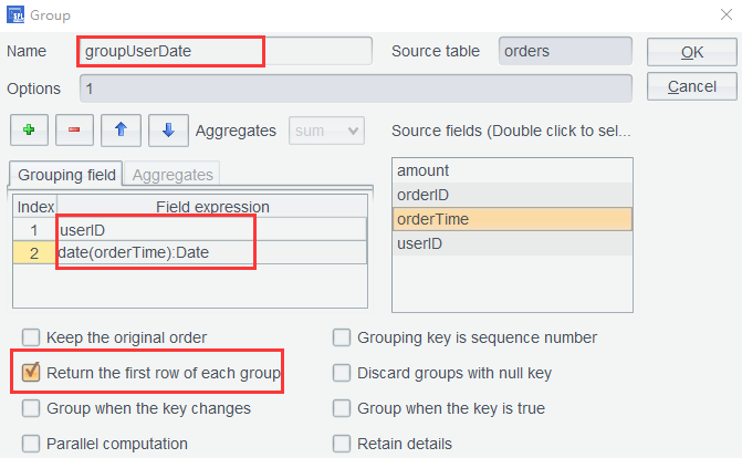
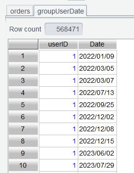
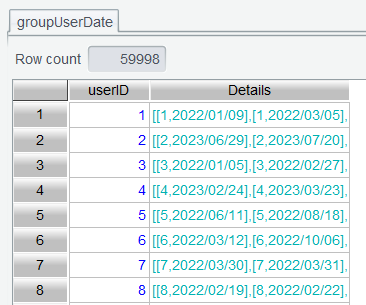
If there are multiple orders in the same day, check Return the first row of each group to remove duplicates. By checking this option, the aggregation becomes meaningless. So, the aggregation settings in the above screenshot are disabled. Click OK to get a table containing user order dates:

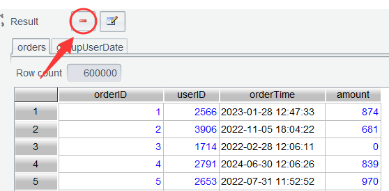
The subsequent analysis only needs the groupUserDate table. Select orders , click Delete icon and delete it to release memory space:

Step 2: Group groupUserDate by userID and check Retain details:

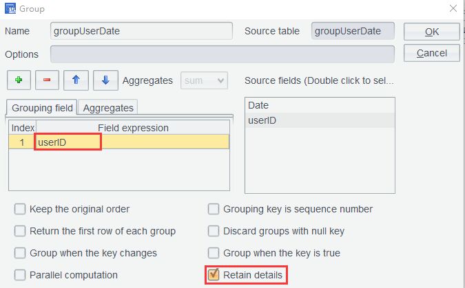
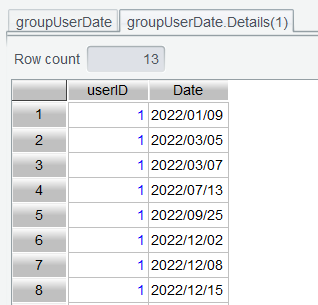
Click OK and get a details table for each userID :

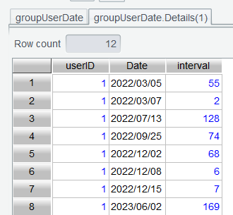
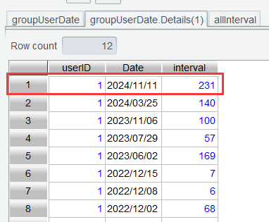
Step 3: Double-click to open the details table under user ID 1:

Use computed column expression interval(Date[-1],Date) to compute purchase interval:

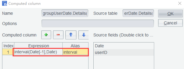
The interval() function gets interval between two dates; the default unit of the returned value is day. Click OK to compute the interval value:

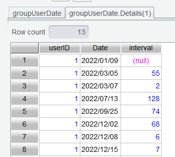
There aren’t any rows before the first data row, so its interval value is null. On the filtering interface we use expression interval!=null to remove this row:

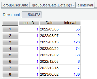
Step 4: Perform Concatenate details data on groupUserDate table to concatenate all records as allInterval :

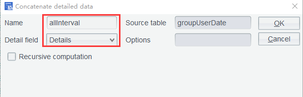
Click OK to get the concatenation result:

Step 5: Now we find the last purchase data row for each user. Back to groupUserDate.Details(1) , where we use interface-based sorting to sort rows by date in descending order. Note: operations on a details table will be synced to each of the other details tables only when they are performed through icons. If you double-click the column header to sort, only the current details table will be ordered.

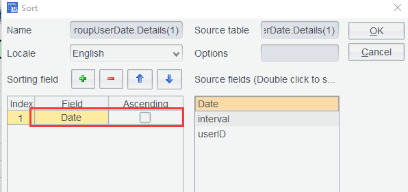
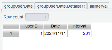
Click OK to perform the sorting, and the last purchase data row is moved to the first row:

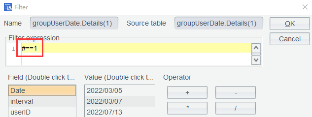
Use filter expression #==1 to retain the last purchase data row and remove the other rows for each user:

The result where only the last purchase data row is retained:

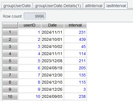
Step 6: Back to groupUserDate to use Concatenate details data again:

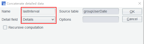
Click OK to get a table consisting of each user’s last purchase data row:

Step 7: In Edit Command Zone, execute allInterval.avg(interval) to compute average purchase interval of all users:

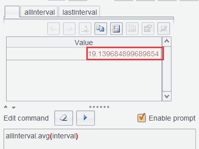
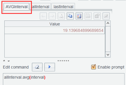
This value will be used in expressions in the subsequent computation. Since a result set obtained from executing a command in the Edit Command Zone by default does not have a name, we need to give it a name for later reference. As Section 3.8 does, we name it AVGInterval :

In lastInterval table, find customers who do not make a repeat purchase after the average purchase interval time is passed. The current order data is as of the end of 2024, so the above expression computes the average purchase interval before the last day of 2024.

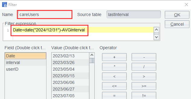
Click OK to get customers for which a win-back strategy needs to be planned:

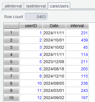
By comparing the table’s row count with the row count in lastInterval , we find that more than half of the customers need special attention, which aligns well with our analytical expectations.