4.1 Data information

Open esProc, run createOrders.splx, and you can get below data table.

This is a supermarket orders data table (orders.csv). It has the following fields:

Column name	Description
orderID	Order ID
userID	User ID
orderTime	Order date
amount	Order amount

This table stores the supermarket’s orders records, a total of 6 million, in three years from 2022 to 2024. It has only several fields and thus can be loaded to generally any ordinary laptop. So, the algorithms introduced in this chapter are all based on in-memory computations.

4.2 Compute sales amount by year and month

	A
1	=file(“orders.csv”).import@tc(orderTime,amount)
2	=A1.groups(year(orderTime):Year,month(orderTime):Month;sum(amount):TotalAmount)

A1 Read data of orderTime field and amount field from orders.csv. Specifying fields to be retrieved in import() function helps reduce memory usage.

A2 Group A1 by year and month and compute sales amount in each group. Again, we emphasize that a year and a month expression can directly act as grouping expressions.

Below is the result of executing A2’s statement:

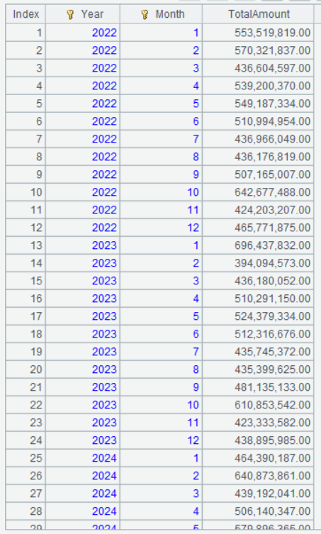
It can be seen that the grouping & aggregation result set is automatically ordered by the grouping expressions. In the next section where this way of orderliness is needed, there is no need to perform sorting again.

4.3 Compute MoM sales growth rate

	A
1	=file(“orders.csv”).import@tc(orderTime,amount)
2	=A1.groups(year(orderTime):Year,month(orderTime):Month;sum(amount):TotalAmount)
3	=A2.derive((TotalAmount-TotalAmount[-1])/TotalAmount[-1]:MoM)

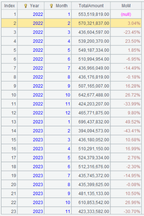
A3 Since A2’s data is already ordered by year and month, we directly use operator [-1] to get TotalAmount value in the preceding row to compute the MoM growth rate. The meaning of the operator was already explained the previous learning point.

Below is result of executing A3’s statement:

Learning point: What is Month-over-Month Growth Rate?

Month-over-Month Growth Rate is the percent change in a certain metric from one time period (usually month or quarter) to the next neighboring period. It is used to measure the changes of trend in a relatively short period.

• Calculation formula:

MoM Growth Rate=(value of the current period−value of the preceding period)/value of the preceding period

• Key characteristics:
  • Between consecutive time periods: Neighboring time periods will be compared (like the current month vs. the preceding month, the current quarter vs the preceding quarter).
  • Short-term fluctuations reflected: Suitable for analyzing seasonal or short-term trend, and abrupt change (such as sales change thanks to holiday promotion).
  • Greatly affected by seasons: For example, in the retail industry the MoM growth rate in December (the Christmas and New Year season) is probably significantly higher than those in the other months.

4.4 Compute YoY growth rate

Method 1: Since supermarket sales data is generated in each month without any interruption, we can use [-12] to obtain data of the same month in the last year：

	A
1	=file(“orders.csv”).import@tc(orderTime,amount)
2	=A1.groups(year(orderTime):Year,month(orderTime):Month;sum(amount):TotalAmount)
3	=A2.derive((TotalAmount-TotalAmount[-12])/TotalAmount[-12]:YoY)

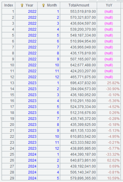
A3 TotalAmount[-12] gets data of the same month in the last year. The meaning of [-12] is already introduced in the previous learning point.

Below is result of executing A3’s statement:

Method 2: Group records by month and year, and then we can use [-1] to obtain data of the same month in the last year. This, together with if judgment, finds if the current month/year and the preceding one are the same:

	A
1	=file(“orders.csv”).import@tc(orderTime,amount)
2	=A1.groups(month(orderTime):Month,year(orderTime):Year;sum(amount):TotalAmount)
3	=A2.derive(if(Year[-1]==Year-1 && Month[-1]==Month, (TotalAmount-TotalAmount[-1])/TotalAmount[-1], null):YoY)

A2 Sort records by month and year.

A3 Use if judgement. If the year in the preceding row is equal to “the current year -1” and the month in the preceding row is the same as the current one, use expression (TotalAmount-TotalAmount[-1])/TotalAmount[-1] to compute YoY growth rate; otherwise return null.

Learning point: What is Year-over-Year (YoY) Growth Rate?

YoY Growth Rate is the change percentage in a certain metric between same time periods in two different years. It is used to show the long-term trend by getting rid of the seasonal effects.

• Calculation formula:

YoY Growth Rate=(value of the current period−value of the same period in last year)/value of the same period in last year

• Key characteristics:
  • Between same time periods: Same time periods in different years are compared (such as Q1 of 2024 vs. Q1 of 2023).
  • Seasonal factors eliminated: Better reflect real growth potential by avoiding interferences from seasonal factors such as holidays and climate.
  • Long-term trend displayed: Suitable for analyzing annual growth, industry life cycle and policy effects.

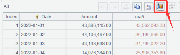
4.5 Compute 5-day moving average

	A
1	=file(“orders.csv”).import@tc(orderTime,amount)
2	=A1.groups(date(orderTime):Date;sum(amount):Amount)
3	=A2.derive(Amount[-2:2].avg():ma5)

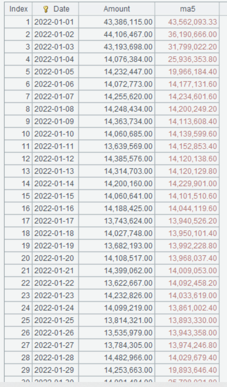
A2 Group records by date and compute daily total sales.

A3 Amount[-2:2] represents a set of Amount field values in five rows - from preceding two rows of the current one to the next two rows of the current one. .avg() computes average value on the set.

Below is result of executing A3’s statement:

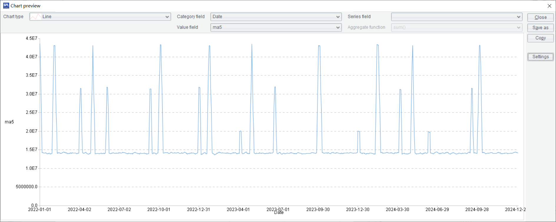
Click Graph icon at the upper right corner:

Select Line chart, Date for Category and ma5 for Value, and click Settings button to get the following pop-up windows:

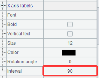
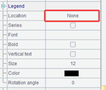
Set 90 as x axis label interval and None for location, and the following chart is dispalyed:

Learning point: What is Amount[-2:2]?

In esProc SPL,Amount[-2:2] references a range of Amount field values based on relative positions, showing a powerful sliding window reference syntax.

Starting from the current record, Amount [-2:2] gets a subset of values from its preceding two records to its next two records (including the current record). This reference method is particularly suitable for dealing with analytical scenarios involving contextual data, such as sliding window computation and moving average computation.

• Basic characteristics:

  • Window definition: [start offset:end offset]defines the relative position-based window.
  • Boundary included: Include records where the offset starts and where it ends.
  • Dynamic window: The window size is fixed but contents vary based on position of the current record.
  • Auto truncation: Automatically truncate the window when it exceeds the boundary of the currently handled sequence.

• Example table:

Row number	Month	Amount
1	Jan	100
2	Feb	120
3	Mar	150
4	Apr	130
5	May	160

• Computing process of Amount[-2:2]:

Current row	Value of Amount[-2:2]	Positions of records covered by the window
Record of Jan	[100,120,150]	Rows 1-3; there isn’t any row before the current one.
Record of Feb	[100,120,150,130]	Rows 1-4; there is only one row before the current one.
Record of Mar	[100,120,150,130,160]	Rows 1-5, which form a complete -2:+2 window.
Record of Apr	[120,150,130,160]	Rows 2-5; there is only one row after the current one.
Record of May	[150,130,160]	Rows 3-5, there isn’t any row after the current one.

• Boundary handling:

  • Start boundary: The window automatically shrinks when there isn’t enough number of records before the current one.
  • End boundary: The window automatically shrinks when there isn’t enough number of records after the current one.
  • Empty window: May return an empty sequence in the extreme case.
  • Asymmetric window: Support asymmetric windows like Amount[-3:1].

• Application scenarios:

Such a flexible window-style reference mechanism enables SPL to achieve complicated sliding-window analyses using very concise syntax, including:

• Moving average computation
  • Rolling statistics
  • Comparison analysis between neighboring records
  • Local trend analysis
  • …

Learning point: What is moving average?

A moving average is a statistical method employed to analyze time series data. It smoothens short-term fluctuations by computing average value within a certain time window and thus helps observe the long-term trend. The method is widely used in various industries and fields, including financial fields, economic study, meteorology, quality control, and so on.

• Key concepts:

  • Smooth data: Eliminate short-term noises (such as price fluctuations and random errors) to highlight the key trend.
  • Time window: Compute average value in a certain period of time (such as 5 days, 20 days and 200 days). The bigger the time window, the smoother the curve but the more unresponsive to recent changes.

• Calculation formula: MAn=(p1+p2+⋯+pn)/n

Where pn is data of the nth day (such as closing price) and n is the window size (such as 5 days).

• Application scenarios:
  • Stock moving average computation: Compute 5-day average (short-term), 20-day average (medium) and 200-day average (long-term). The stock moving average is computed by averaging past data, such as [-5:-1] and [-19:-1], which are asymmetric time windows. SPL is particularly good at computing average on such a window, without needing a special function.
  • Economic statistics: Smooth seasonal indicator fluctuations, such as GDP and unemployment rate.
  • Meteorology: Handle short-term fluctuations of temperature and precipitation.

4.6 Compare weekday sales and weekend sales

Method: Group records by date, compute the day corresponding to each date, select records of weekends and those of weekdays, and compute daily average sales respectively to get the comparison result.

	A
1	=file(“orders.csv”).import@tc(orderTime,amount)
2	=A1.groups(date(orderTime):Date;sum(amount):Amount)
3	=A2.derive(day@w(Date):weekday)
4	=A3.select(weekday==1 || weekday==7)
5	=(A3\A4)
6	=A4.avg(Amount)
7	=A5.avg(Amount)

A3 Add a computed column to find what day each date is. day@w(Date) gets the day corresponding to the Date.

A4 Get records where the day is 1 or 7, which corresponds to Sunday or Saturday.

A5 Get records that do not exist in A4 from A3, that is, return records of weekdays. The slash symbol ()represents a difference operation between sequences (sets).

A6 and A7 respectively compute daily average sales during weekdays and the weekend.

The computing result shows that daily average sales during the weekend is much higher than that during the weekdays. According to this, additional staff can be provided on weekend.

4.7 Find the proportion of sales of a certain time period

Method: Group sales records by hour, compute hourly average sales then the proportion of it in the total sales of the day. This shows the peak and trough of sales. Considering the difference between weekend and weekdays, records of them are summarized respectively:

	A
1	=file(“orders.csv”).import@tc(orderTime,amount)
2	=A1.groups(date(orderTime):Date,hour(orderTime):Hour;sum(amount):Amount)
3	=A2.select([1,7].pos(day@w(Date)))
4	=(A2\A3)
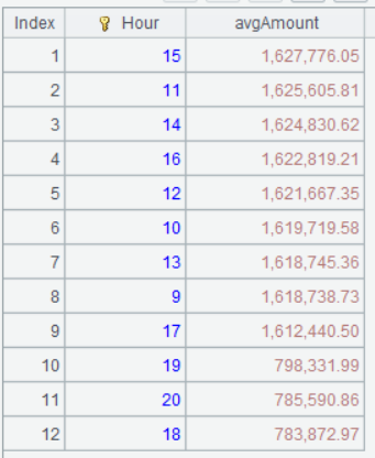
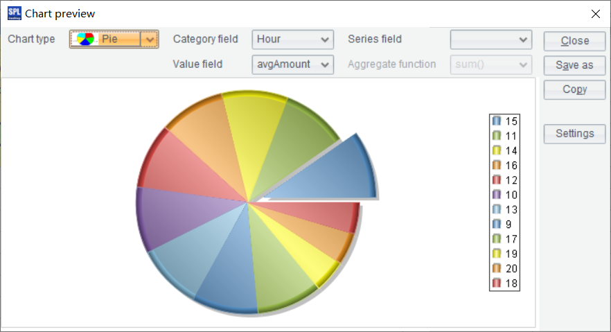
5	=A3.groups(Hour;avg(Amount):avgAmount).sort(-avgAmount)
6	=A4.groups(Hour;avg(Amount):avgAmount).sort(-avgAmount)

A2 Group records by date and hour and compute total sales in each group.

A3 Get records where the day is 1 or 7, that is, records of weekends. [1,7].pos(day@w(Date)) finds whether the day computed through day@w(Date) is contained in set [1,7] and, return the corresponding sequence number if it is a member, or return null it isn’t.

A5 Group records by hour, compute average weekend sales in each hour, and sort records.

A6 Group records by hour, compute average weekday sales in each hour, and sort records.

Below is result of computing A5’s statement:

Below is result of computing A6’s statement:

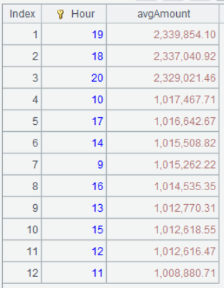
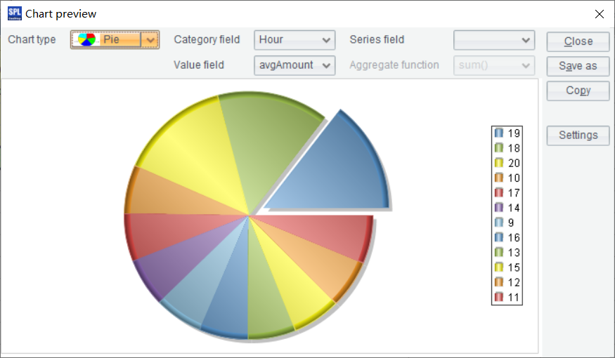
According to the above chart, the sales peak comes from 18 o’clock to 21 o’clock during weekdays, while the peak is from 9 o’clock to 18 o’clock on weekend. Sellers can change their business hours or optimize the resources (such adding additional staff at the peak hours) according to the finding.

4.8 Track sales completion rate

Suppose the monthly average sales is set as sales target of a month and we want to compute the daily cumulative sales completion rate in October of the year 2024.

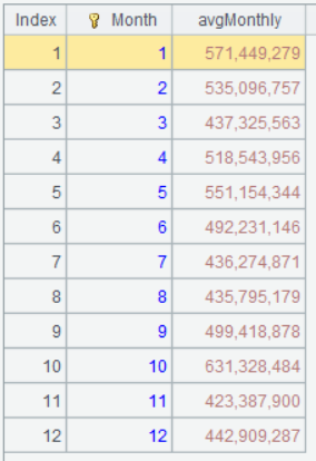
Step 1: Compute monthly average sales.

	A
1	=file(“orders.csv”).import@tc(orderTime,amount)
2	=A1.groups(year(orderTime):Year,month(orderTime):Month;sum(amount):TotalAmount)
3	=A2.groups(Month;avg(TotalAmount):avgMonthly)

A2 Group records by year and month, and compute monthly sales.

A3 Group and summarize records by month to find the monthly average sales, which is sales target of the month.

Below is result of executing A3’s statement:

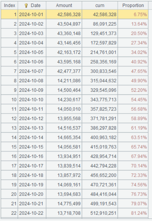
Step 2: Select records of October in the year 2024, group and summarize them by date to get the daily sales, compute the cumulative amount, and divide the target sales by the cumulative sales to get the sales completion rate of the current date.

	A
4	=A1.select(year(orderTime)==2024 && month(orderTime)==10)
5	=A4.groups(date(orderTime):Date;sum(amount):Amount)
6	=A5.derive(cum[-1]+Amount:cum,cum/A3(10).avgMonthly:Proportion)

A4 Select records of October in 2024.

A5 Group and summarize records by date to compute daily sales.

A6 cum[-1]+Amount adds the current sales amount to the preceding day’s cumulative amount to get the cumulative sum of the current date. cum/A3(10).avgMonthly divides target sales of October by the current date’s cumulative amount to get the current date’s cumulative sales completion rate. A3(10) gets the 10^th record from A3, and A3(10).avgMonthly gets avgMonthly field value of the record.

Below is result of executing A6’s statement:

4.9 Repurchase cycle analysis

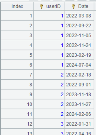
Step 1: Retrieve unique records by user ID and order date. Users’ multiple orders are regarded as purchases of missing items or order splitting for obtaining discounts rather than repurchases. So, distinct operation on date is performed.

	A
1	=file(“orders.csv”).import@tc(userID,orderTime)
2	=A1.groups(userID,date(orderTime):Date)

A1 Retrieve userID field and orderTime field from orders.csv.

A2 Group records by UserID and date(orderTime). As no aggregate expression is specified in the groups() function, it performs distinct on the grouping fields.

Below is result of executing A2’s statement:

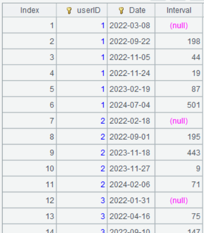
Step 2: Compute interval between repurchases.

	A
3	=A2.derive(if(userID[-1]==userID,interval(Date[-1],Date),null):Interval)

A3 if(userID[-1]==userID,interval(Date[-1],Date),null) computes the number of days between the date of the preceding record and the date of the current record when userID in the preceding record is the same as that in the current record it, and returns null when they are not same. interval() function computes the interval between two dates; the unit of the value it returns is by default the day.

Below is result of executing A3’s statement:

Step 3: Compute average interval between purchases.

	A
4	=A3.select(Interval)
5	=A4.avg(Interval)

A4 Select records where Interval value isn’t null.

A5 Compute average number of days between purchases.

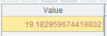
Below is result of executing A5’s statement:

Step 4: Select users whose last purchase date is earlier than the day directly before “average interval between purchases” days.

	A
6	=now@d()-A5
7	=A2.group@o(userID).(~.m(-1))
8	=A7.select(Date<A6)

A6 now@d() returns the current date, without including the time component. now@d()-A5 gets the date directly before the “average interval between purchases” days. SPL allows directly using the minus/plus sign to get the date n days before/after.

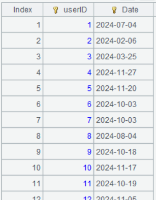
A7 Group A2 by userID and select the last record from each group, which corresponds to the date when the current user makes the last purchase. ~.m(-1) gets the last record from the current group.

A8 Select records where the date is earlier than A6. They are the users whose current purchase interval has exceeded the average repurchase cycle, and for them a re-engagement strategy needs to be made.

Below is result of executing A7’s statement: