3.1 Compute total sales of each salesperson in the last year

	A
1	=file(“sales.csv”).import@tc(sales,orderDate,quantity,price,discount)
2	=A1.select(year(orderDate)==2024)
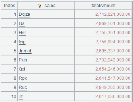
3	=A2.groups(sales;sum(quantity*price*discount):totalAmount)

A3 A2.groups(sales;sum(quantity*price*discount):totalAmount) groups record sequence A2 by sales, compute aggregate expression sum(quantity*price*discount) while naming the result totalAmount, and returns a table sequence made up of two fields – sales, totalAmount. It basically amounts to SQL statement "select sales, sum(quantity*price*discount) as totalAmount from A2 group by sales ".

In the previous sections, we mentioned sum, max, min, count, icount and other aggregate functions. Each of them can be used in an aggregate expression in the groups() function.

In this example, the aggregate expression is sum(orderAmount). The order amount is computed through expression quantity*price*discount directly in the sum() function without adding a computed column in advance.

One thing you need to particularly note is that the grouping field and the aggregate expression are separated by semicolon and that the aggregate expression and the corresponding column name are separated by colon. The rule is the same as that for the above-mentioned derive() function.

Result of executing A3’s statement:

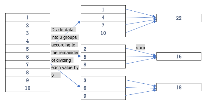
Learning point: What is grouping operation?

A grouping operation divides data into multiple groups according to a specified rule and performs a certain aggregate operation on each group of data using an aggregate expression. For example:

3.2 Compute proportion of each seller’s sales to the total

	A
1	=file(“sales.csv”).import@tc(sales,orderDate,quantity,price,discount)
2	=A1.select(year(orderDate)==2024)
3	=A2.groups(sales;sum(quantity*price*discount):totalAmount)
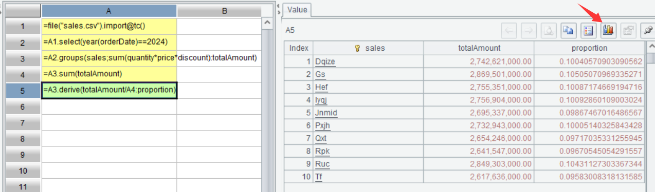
4	=A3.sum(totalAmount)
5	=A3.derive(totalAmount/A4:proportion)

A4 Compute total sales amount in the whole year.

A5 Add a computed column to get proportion of each seller’s sales to the whole year total.

On the interface, select A5 and click Browse graphics button on the Value viewing section on the right:

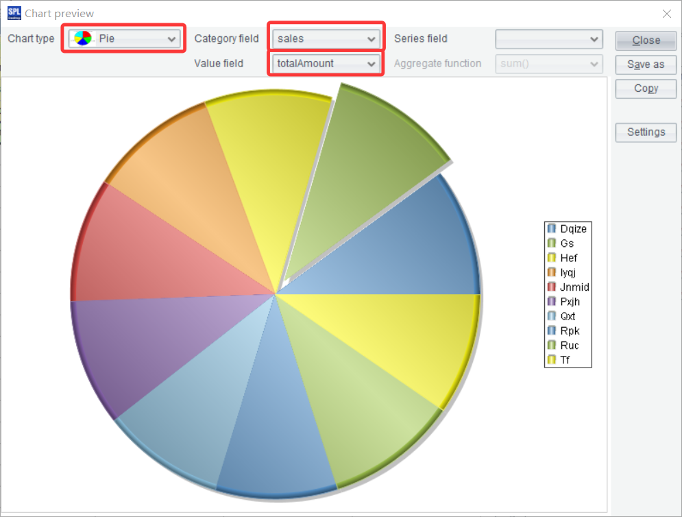
On the pop-up interface, select Pie for Chart type, sales for Category field and totalAmount for Value field, and a pie chart is plotted to visually display proportions of amounts of different sellers to the total:

3.3 Find sellers whose sales amounts rank in top3

	A
1	=file(“sales.csv”).import@tc(sales,orderDate,quantity,price,discount)
2	=A1.select(year(orderDate)==2024)
3	=A2.groups(sales;sum(quantity*price*discount):totalAmount)
4	=A3.top@r(3,-totalAmount)

A4 Compute rankings according to A3’s grouping result and return sellers whose sales amounts rank top3.

3.4 Find the bestselling products in the last year (by frequency)

	A
1	=file(“sales.csv”).import@tc(orderDate,product)
2	=A1.select(year(orderDate)==2024)
3	=A2.groups(product;count(1):num)
4	=A3.top@r(1,-num)

A3 Group data by product and count the number of purchases.

A4 Get all products with the most number of purchases. To select those ranked first or last, you can also use =A3.maxp@a(num) or minp@a, which returns the same result.

3.5 Compute total sales and quantity for each seller by year

	A
1	=file(“sales.csv”).import@tc(sales,orderDate,quantity,price,discount)
2	=A1.groups(year(orderDate):oYear,sales;sum(quantity):totalQuantity, sum(quantity*price*discount):totalAmount)

A2 The expression syntax for grouping & aggregation by multiple fields is similar to that by a single field. The multiple fields are separated by comma. Note that when a grouping expression instead of a grouping field is specified, you can perform the grouping directly according to the expression without first using derive() to add a computed column to the table sequence. year(orderDate):oYear in the above script, for example, means grouping by year(orderDate) and naming result field oYear.

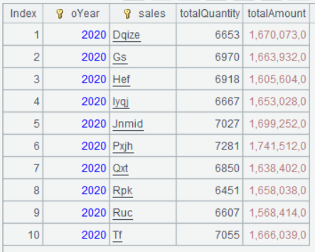
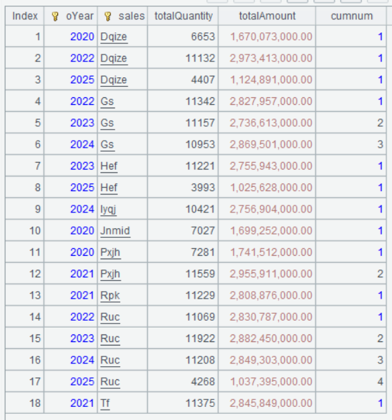
Below is the result of executing A2’s statement:

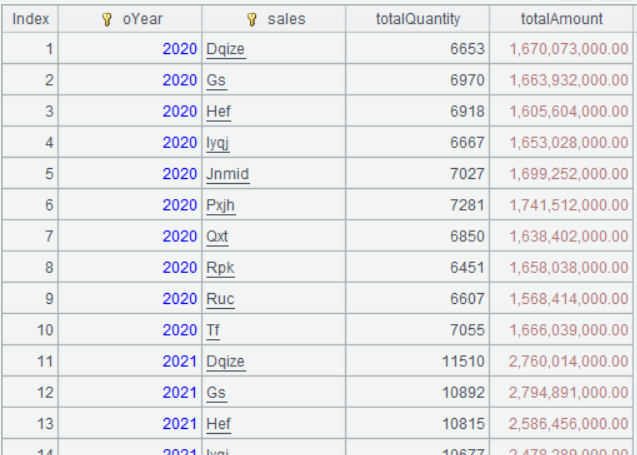
Evidently, the result of groups() is a table sequence containing grouping expression values and aggregate expression values.

3.6 For each year, get salespeople whose sales amounts rank in top3

The more intuitive method: perform grouping operation by year and get sellers who rank in top3 from each group. This requires that after grouping each subset of details data can be retained, because only with the subsets can the top3 sellers be obtained.

As the screenshot below shows, data highlighted in red box is the details in each group:

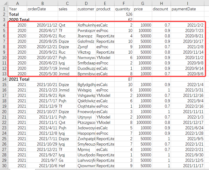
By looping through each group of details data to perform the computation, it is easy to get the top 3 in each year.

SPL has group() function, which can group data while retaining each subset of data:

	A
1	=file(“sales.csv”).import@tc(sales,orderDate,quantity,price,discount)
2	=A1.groups(year(orderDate):oYear,sales;sum(quantity):totalQuantity, sum(quantity*price*discount):totalAmount)
3	=A2.group(oYear)

A3 Group A2 by oYear field and return each subset of data.

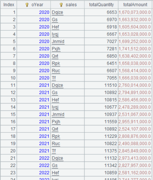
Below is result of executing A2’s statement:

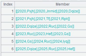
Below is result of executing A3’s statement:

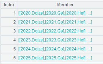
Data is divided into six groups by year. Click a group and you can see the corresponding data set:

Having every subset of data, you can compute to find the top3 in each group:

	A
1	=file(“sales.csv”).import@tc(sales,orderDate,quantity,price,discount)
2	=A1.groups(year(orderDate):oYear,sales;sum(quantity):totalQuantity,sum(quantity*price*discount):totalAmount)
3	=A2.group(oYear)
4	=A3.(~.top@r(3;-totalAmount))

A4 A3.(~.top@r(3;-totalAmount)) performs loop operation on A3. Within the loop body, ~.top@r(3;-totalAmount) finds sellers ranked in top3 in terms of sales amount in each group; ~ represents the currently looped member in A3. Since A3 is a set consisting of grouped sets, ~ is the currently looped group.

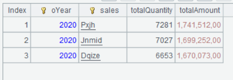
Below is result of executing A4’s statement:

Click a row and you see the top3 in the group:

Learning point: What is ~?

In SPL, a tilde (~) is used to reference the current member. During a loop operation on a sequence or a sequence of tables, ~ represents the currently handled member object. In a loop function (such as sum(), select() and group()), ~ directly references the current element, which simplifies the syntax of set operations.

Typical use case:

	A
1	=[1,2,3,4]
2	=A1.(~*~)
3	=file(“sales.csv”).import@tc()
4	=A3.select(~.quantity>5)
5	=A3.select(quantity>5)

A2 Compute square of each element in A1’s sequence.

A4 Select records where quantity is greater than 5 from A3. The syntax is equivalent to that in A5.

Technique description:

• Contextual valuation: The value of ~ is decided by the context of currently executed iteration.
• Dynamic reference: In a multilayer iteration, ~ always points to the current element in the innermost loop.
• Various value type: ~ can represent a value of a simple data type, or an object such as record and sequence.
• Simplified expression: ~ can be omitted when a field name is also used, such as ~.quantity, which can be simplified as quantity. In all the previous examples, ~ is omitted and the simplified form is used.

SPL’s tilde syntax makes the language’s structured data processing code particularly concise and significantly increases its description efficiency.

3.7 Get the salesperson who most frequently ranked in top3

Now we have the result of the preceding example. If you want to find the salesperson who most frequently appears in the top3 rankings, just concatenate the result records into a record sequence, group and count records by sales, and return the record having the largest count.

Step: Concatenate every year’s records ranked in top3 into a record sequence.

	A
1	=file(“sales.csv”).import@tc(sales,orderDate,quantity,price,discount)
2	=A1.groups(year(orderDate):oYear,sales;sum(quantity):totalQuantity, sum(quantity*price*discount):totalAmount)
3	=A2.group(oYear)
4	=A3.(~.top@r(3;-totalAmount))
5	=A4.conj()

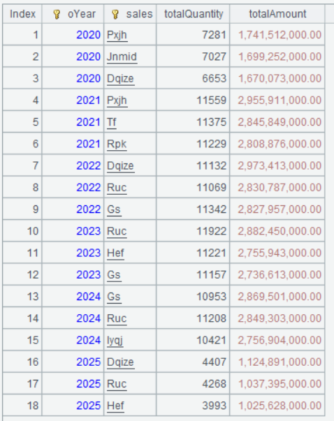
A5 A4.conj() concatenates A4’s set of groups into a record sequence. According to the preceding example, A4’s result is a set of sets. The conj() function flattens the two-layer set into a single one. Below is A5’s result:

Step 2: Group records by sales, perform count operation on each group, and select the record having the largest count:

	A
1	=file(“sales.csv”).import@tc(sales,orderDate,quantity,price,discount)
2	=A1.groups(year(orderDate):oYear,sales;sum(quantity):totalQuantity, sum(quantity*price*discount):totalAmount)
3	=A2.group(oYear)
4	=A3.(~.top@r(3;-totalAmount))
5	=A4.conj()
6	=A5.groups(sales;count(1):num)
7	=A6.maxp@a(num)

Uses of both groups() function and maxp@a function are already illustrated, and we just skip them.

3.8 Get the salesperson who ranked in top3 in consecutive 3 years

The intuitive way of handling this task is this:

Sort records of the yearly salespeople who ranked in top3 by sales and the year and perform accumulative sum. For the same salesperson and if one year is passed, the accumulative sum is 1; otherwise perform the count anew starting from 1. Lastly, select records where the accumulative count is 3.

Step1: Sort records by sales and the year:

	A
1	=file(“sales.csv”).import@tc(sales,orderDate,quantity,price,discount)
2	=A1.groups(year(orderDate):oYear,sales;sum(quantity):totalQuantity,sum(quantity*price*discount):totalAmount)
3	=A2.group(oYear)
4	=A3.(~.top@r(3;-totalAmount))
5	=A4.conj()
6	=A5.sort(sales,oYear)

Step 2: Add a computed column, where the count value starts from 1. If the salesperson of the current row is still the one in the preceding row and the current row’s year is equivalent to the preceding row’s year + 1, add 1 to the current count; otherwise count anew from 1.

	A
1	=file(“sales.csv”).import@tc(sales,orderDate,quantity,price,discount)
2	=A1.groups(year(orderDate):oYear,sales;sum(quantity):totalQuantity, sum(quantity*price*discount):totalAmount)
3	=A2.group(oYear)
4	=A3.(~.top@r(3;-totalAmount))
5	=A4.conj()
6	=A5.sort(sales,oYear)
7	=A6.derive( if(sales==sales[-1] && oYear==oYear[-1]+1, cumnum=cumnum[-1]+1, cumnum=1):cumnum )
8	=A7.select(cumnum==3)

A7 sales[-1] represents sales field value in the preceding row; and sales[1] represents sales field value in the directly next row. if(sales==sales[-1] && oYear==oYear[-1]+1, cumnum=cumnum[-1]+1, cumnum=1) function executes cumnum=cumnum[-1]+1 when the value of boolean expression sales==sales[-1] && oYear==oYear[-1]+1 is true, otherwise it executes cumnum=1. Here if() function works according to the same rules as its Excel counterpart.

A8 Select all records whose cumnum is 3.

Below is result of executing A7’s statement:

Below is result of executing A7’s statement:

This way the salespeople who ranked in top3 in consecutive 3 years are selected.

Learning point: What is sales[-1]?

sales[-1] references sales field value in the preceding record of the current one; conversely, sales[1] references sales field value in the next record of the current one. They are the relative position-based reference syntax unique to the SPL language. The syntax applies in scenarios where neighboring values or records need to be accessed.

Basic characteristics:

• Relative location: Access data according to the current record’s relative position.

• Dynamic computation: The specific value to be referenced is determined by location the currently processed row.

• Boundary processing: When the reference is beyond the sequence (like the preceding row of the first one or the next row of the last one), null is returned.

Typical application scenarios:

• Compute YoY/MoM growth

• Query neighboring record

• Achieve sliding window computation

Illustration

• Example data table

Month	sales
Jan	100
Feb	120
Mar	150
Apr	130

• Computing process of sales[-1] and sales[1]

Current processed row	Value of sales[-1]	Value of sales[1]	Computing logic of sales[-1]	Computing logic sales[1]
Record of Jan	null(no preceding row)	120	[no preceding record]	Get sales value of Feb
Record of Feb	100	150	Get sales value of Jan	Get sales value of Mar
Record of Mar	120	130	Get sales value of Feb	Get sales value of Apr
Record of Apr	150	null(no next row)	Get sales value of Mar	[no next record]

Boundary processing

• For the first record: sales[-1]returns null

• For the last record: sales[1]returns null

• Cross-group reference: In a grouping operation, relative position-based reference only occurs within the current group

• Multilevel offset: It also supports syntax such assales[-2](preceding 2 records) and sales[3](next 3 records)

The relative position-based reference mechanism helps produce concise and intuitive expressions in handling time series computation and sliding window analysis.

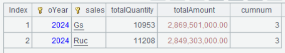
3.9 Among salespeople whose sales amounts ranked in top3 in 2025, find the one who gets the most consecutive appearances in yearly top3 rankings

With the result of the preceding computing task, you just need to select from A7 the one where cumnum value is the largest from records of the year 2025:

	A
1	=file(“sales.csv”).import@tc(sales,orderDate,quantity,price,discount)
2	=A1.groups(year(orderDate):oYear,sales;sum(quantity):totalQuantity, sum(quantity*price*discount):totalAmount)
3	=A2.group(oYear)
4	=A3.(~.top@r(3,-totalAmount,~))
5	=A4.conj()
6	=A5.sort(sales,oYear)
7	=A6.derive(if(sales==sales[-1] && oYear==oYear[-1]+1,cumnum=cumnum[-1]+1, cumnum=1):cumnum)
8	=A7.select(oYear==2025).maxp@a(cumnum)

3.10 Aggregation by different amount ranges

Suppose we divide order amounts into three ranges - ≥5 million, ≥1 million and＜5 million, and＜1 million, and respectively count large, medium and small orders and sum their amounts.

	A
1	=file(“sales.csv”).import@tc(sales,orderDate,quantity,price,discount)
2	=A1.select(year(orderDate)==2024).derive(quantity*price*discount:amount)
3	=A2.groups(if(amount>=5000000:"B",amount>=1000000:"M";"S"):type; count(1):oNum, sum(amount):oAmount)

A3 Group and summarize A2 by order amount ranges. Here the parameter rule in if() function is different from what we explained previously. The meaning of if(amount>=5000000:"B",amount>=1000000:"M";"S") is that when condition amount>=5000000 is met, the function returns "B"; and when amount>=1000000 is met, it returns "M"; otherwise the function returns "S". This amounts to the two-layer statement if(amount>=5000000,"B", if(amount>=1000000, "M","S")). As such a statement is commonly used, SPL specifically provides a simplified form.

Below is the result of computing A3’s statement:

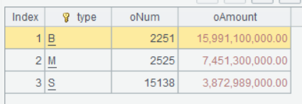
You can see that small orders are the most in number, but their total amount is the smallest. The number of large orders and that of medium orders are nearly the same, but the former’s total is far more than the latter’s.