Traditional transactional databases (TP) do not good at handling analytical computations. Professional OLAP databases are too heavy and often need clustering, resulting in high costs and more complicated system structure.

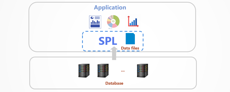
Storing static historical data as a lightweight esProc SPL file of columnar format enables access to SPL’s powerful computing capabilities, producing far better performance than traditional databases generate. esProc SPL is lightweight, and can run by being directly embedded in the application. It can speed up queries on dumped data while maintaining a relatively simple system structure.

This article provides a series of practical SPL methods for speeding up external data querying:

Practice #1: Regular Filtering and Grouping & Aggregation

Practice #2: COUNT DISTINCT

Practice #3: Foreign-key-based Dimension Table Join

Practice #4: Large Primary-Subtable Join

Practice #5: EXISTS at Large Primary-Subtable Join

Practice #6: Conditional Filtering by Enumerated Field

Examples in these articles cover operations having performance issues that have greatly troubled traditional databases. Those include COUNT DISTINCT, foreign-key-based JOIN, large primary-subtable JOIN (including EXISTS), conditional filtering by enumerated field (including IN), to name a few. These articles will help you break database query performance bottlenecks.

Some preparation work is required before we start.

【Here】 we have csv files and a create table SQL file to simulate part of the data of a company’s offline orders and e-commerce activities. The goal is to create tables in MYSQL database and import data from the csv files into them.

Below is the relationship between the preceding csv files:

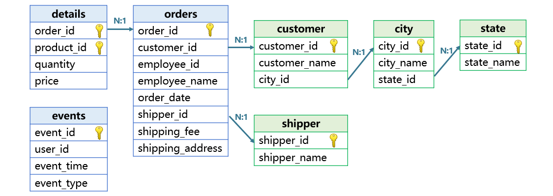
The event table (events) stores users’ actions on the e-commerce website in ten million rows and the following fields:

Fields	Description	Type	Note
event_id	Event ID	Integer	Primary key
user_id	User ID	Integer	About one million IDs
event_time	Time when an event happens	Datetime	Within the year 2025
event_type	Event type	Integer	1 represents login, 2 represents view, …, and 7 represents confirm

Orders table (orders) stores offline orders data in ten million rows:

Fields	Description	Type	Note
order_id	Order ID	Integer	Primary key
customer_id	Customer ID	Integer
employee_id	Employee ID	Integer
employee_name	Employee name	String
order_date	Date when an order is placed	Date	Within the year 2024
shipper_id	Shipper ID	Integer
shipping_fee	Shipping fee	Numeric
shipping_address	Shipping address	String

Orders detail (details) stores offline orders details in thirty million rows:

Fields	Description	Type	Note
order_id	Order ID	Integer	Primary key
product_id	Product ID	Integer	Primary key
quantity	Order quantity	Integer
price	Unit Price	Numeric

Customer table (customer) stores data of offline customers. The table has a relatively small amount of data:

Fields	Description	Type	Note
customer_id	Customer ID	Integer	Primary key
customer_name	Customer name	String
city_id	City ID	Integer

City table (city) stores data of cities where offline customers are based. The table has a relatively small amount of data:

Fields	Description	Type	Note
city_id	City ID	Integer	Primary key
city_name	City name	String
state_id	State ID	Integer

State table (state) stores data of states where offline customers come from. The table has a relatively small amount of data:

Fields	Description	Type	Note
state_id	State ID	Integer	Primary key
state_name	State name	String

Shipper table (shipper) stores data of offline shippers. The table has a relatively small amount of data:

Fields	Description	Type	Note
shipper_id	Shipper ID	Integer	Primary key
shipper_name	Shipper name	String

Download esProc. The Standard Edition is enough.

After installing esProc, check whether a database can be successfully accessed from IDE. Take MYSQL as an example. Put the database’s JDBC in "[installation directory]\common\jdbc", which is one of esProc’s classpaths:

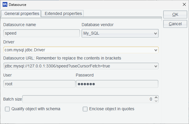
To create MYSQL data source in esProc, select Tool ->Connect to Data Source on the menu, configure the standard MySQL JDBC connection named speed:

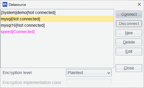
Return to the Datasoure window and connect to the configured data source just now. The setup is successful if the data source name turns pink.

Create a new script in IDE, write SPL statements, and connect to the database to load data from orders table through an SQL statement.

SPL code example 1:

	A
1	=connect("speed")
2	=A1.query@x("select * from orders limit 100")

Press Ctrl-F9 or click the Execute button and then click A2, and there are 100 records listed to the right.

The SPL code is written in the grid, where a cell name can be directly used as a temporary variable.

Look up Tutorial and Function Reference if you have any problems.

The environment where our tests are performed comprises VMware virtual machine, 8-core CPU, 8G RAM, SSD drive, Windows 11 OS, MySQL 8.0, and esProc SPL Standard Edition.