

4.2 Multidimensional combination
4.2.1 Data standardization
In multidimensional time series, different dimensions may have different units of measurement. Before calculating distances, all dimensions need to be standardized to a common scale. The method of converting data with different units to data with a common scale is called ‘data standardization’. In statistics, there are many standardization methods. This book focuses on two common ones: Min-Max scaling (Max_Min) and Standard Score (Z-score).
Let’s have a brief review:
1. Min-Max scaling (Max_Min)
Min-Max scaling performs a linear transformation on the original data. Let mi and ma be the minimum and maximum values of sequence A, respectively. It maps any original value ai of A to a value a’i within the interval [0, 1].
Sequence A
A=[a1,a2,…,an]
Maximum value ma and minimum value mi:
ma=max(A)
mi=min(A)
Min-Max scaling:
a’i=(ai-mi)/(ma-mi)
SPL routine:
| A | B | C | |
|---|---|---|---|
| 1 | [2,4,2,5,10] | /Sequence A | |
| 2 | =A1.max() | ||
| 3 | =A1.min() | ||
| 4 | =d=A2-A3,A1.((~-A3)/d) | /Standardized result | |
2. Standard Score (Z-score)
Z-score standardization standardizes data based on the mean (Ag) and standard deviation (σ) of the original data, transforming the original value ai of sequence A into a’i.
Sequence A:
A=[a1,a2,…,an]
Mean Ag and standard deviation σ:
Ag=avg(A)
σ=std(A)
Z-score standardization:
a’i=(ai-Ag)/σ
SPL routine:
| A | B | C | |
|---|---|---|---|
| 1 | [2,4,2,5,10] | /Sequence A | |
| 2 | =A1.avg() | ||
| 3 | =sqrt(var@s(A1)) | /Standard deviation | |
| 4 | =A1.((~-A2)/A3) | /Standardized result | |
4.2.2 Calculating distances
1. Euclidean distance
Euclidean distance (also known as Euclidean metric) is a commonly used distance metric, representing the straight-line distance between two points in an m-dimensional space.
m-dimensional data points A, B:
A=[a1,a2,…,am]
B=[b1,a2,…,am]
Euclidean distance d between the two points:
d=sqrt(sum((ai-bi)2))
SPL routine:
| A | B | C | |
|---|---|---|---|
| 1 | [3,5,4,12,9] | /Point A | |
| 2 | [5,15,5,6,7] | /Point B | |
| 3 | =dis(A1,A2) | /Euclidean distance | |
2. Mahalanobis distance
Mahalanobis distance is a covariance-based distance, which can be seen as a modification of the Euclidean distance, correcting the issues of inconsistent scales and correlations between different dimensions in the Euclidean distance.
m-dimensional matrix Y:
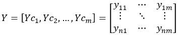
The covariance Cov(Yci,Ycj) between any two columns, Yci and Ycj:
Cov(Yci,Ycj)=sum((yki-avg(Yci))* (ykj-avg(Ycj)))/(n-1),k∈[1,n]
Where yki is the i-th element in the k-th row of matrix Y.
Covariance matrix Σ:
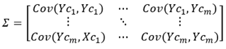
Mahalanobis distance d between points Yri and Yrj in Y:
d=sqrt((Yri-Yrj)T*Σ-1*(Yri-Yrj))
Observing the above equation, it can be found that when the covariance matrix Σ is the identity matrix, the Mahalanobis distance equals the Euclidean distance. When Σ is not invertible, the Mahalanobis distance cannot be computed.
SPL routine:
| A | B | C | |
|---|---|---|---|
| 1 | [[3,5],[5,15],[4,5],[12,6],[9,7]] | /All samples | |
| 2 | [3,5] | /Point A | |
| 3 | [4,5] | /Point B | |
| 4 | =covm(A1) | /Covariance matrix | |
| 5 | =dism(A2,A3,A4) | /Mahalanobis distance | |
Both Euclidean distance and Mahalanobis distance have their respective advantages and disadvantages, as detailed in the table below:
| Advantages | Disadvantages | |
|---|---|---|
| Euclidean distance | Computationally simple; unaffected by the overall sample distribution. | Treats all attributes equally; heavily affected by the units of measurement. |
| Mahalanobis distance | Unaffected by the units of measurement; Eliminates the interference of correlations between variables. |
Affected by the overall sample distribution; distance between two points varies with different sample distributions due to changes in covariance. The covariance matrix must be invertible, otherwise the Mahalanobis distance cannot be computed. |
4.2.3 Anomaly detection
Let Z=Xr[-(k+1)]i+1, where Z is a (k+1)*m matrix, and k is the length of the interval preceding Xri.
1. Compute the pairwise distances between all points in Matrix Z
(1) Euclidean distance
(i) Column standardization
(a) Min-Max scaling
Xcj’=Max_Min(Zcj)
(b) Z-score standardization
Xcj’=Z_score(Zcj)
Where Zcj’ represents the elements of the j-th column in the standardized matrix Z’. Max_Min(…) represents the Max_Min scaling function, and Z_score(…) represents the Z-score standardization function.
(ii) Compute pairwise distances between all points to form the distance matrix DisM:
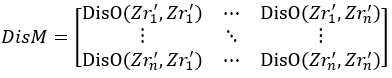
where DisO(…) is the function for computing the Euclidean distance.
(2) Mahalanobis distance
(i) Mahalanobis distance does not require standardization
Z’=Z
(ii) Compute the distance matrix DisM:
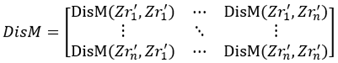
where Dis(…) is the function for computing the Mahalanobis distance.
2. Maximum distance (mdis) in multidimensional space
In multidimensional space, the maximum distance is between the point composed of all dimensions’ maximum values and the point composed of all dimensions’ minimum values.
The coordinates of the point with maximum values for all dimensions:
MaD=[max(Zcj’),j∈[1,m]]
The coordinates of the point with minimum values for all dimensions:
MiD=[min(Zcj’),j∈[1,m]]
Maximum distance mdis
Euclidean distance:
mdis=DisO(MaD,MiD)
Mahalanobis distance:
mdis=DisM(MaD,MiD)
3. Standard radius (r)
r=mdis*r_per
Where r_per is the radius percentage, input as a variable, and the standard radius is defined as the ‘neighborhood’.
4. Number of points within the ‘Neighborhood’ of each point (Dn)
dnl=count(DisMrl<r)
Where dnl represents the number of points within the neighborhood of the l-th point in Z, and DisMrl represents the elements of the l-th row in the distance matrix DisM.
5. Threshold number of points (sn)
sn=Threshold(Dn,arg)
Where Threshold(…) is the threshold calculation function, which can be computed using the box plot method, normal statistical method, or distance method. The resulting lower threshold is used as the threshold number of points. Note: the parameter ‘arg’ must correspond to the respective method. For example, the box plot method requires setting the interquartile range multiplier, the normal statistical method requires setting the standard deviation multiplier, and the distance method requires setting the radius multiplier.
6. Anomaly score (od)
od=if(dnk+1≥Sn,0,(sn-dnk+1)/sn)
The (k+1)-th point in Z corresponds to the i-th point in X. dnk+1 is the number of points within the neighborhood of the (k+1)-th point in Z, and od is the anomaly score of the (k+1)-th point.
| A | B | |
|---|---|---|
| 1 | =file(“2DPlot_data0.csv”).import@tci().to(1000) | /First dimension data |
| 2 | =file(“2DPlot_data1.csv”).import@tci().to(1000) | /Second dimension data |
| 3 | =r_per=0.25 | /Radius percentage (r_per) |
| 4 | =r_n=3 | /Radius multiplier - distance method |
| 5 | =[A1,A2] | /Two-dimensional data |
| 6 | =A5.(Max_Min(~)) | /Min-max normalization |
| 7 | =transpose(A6) | /Transpose |
| 8 | =A7.((idx=#,d=~,A7.m(:idx-1,idx+1:).(dis(~,d)))) | /Distance matrix (DisM) |
| 9 | =A6.(~.max()) | |
| 10 | =A6.(~.min()) | |
| 11 | =dis(A9,A10) | /Maximum distance (mdis) |
| 12 | =A11*r_per | /Standard radius (r) |
| 13 | =A8.(~.count(~<A12)) | /Number of neighborhood points (Dn) |
| 14 | =Threshold(A13,“down”,r_n) | /Threshold number of points (sn) - distance method |
| 15 | =d=A13.m(-1),if(d>=A14,0,1-d/A14) | /Anomaly score (od) |
Any standardization method, distance calculation method, and threshold calculation method described above can be changed. Select better methods and set more suitable parameters based on the specific scenario to adapt to a wider range of industrial applications.
Calculation result example:
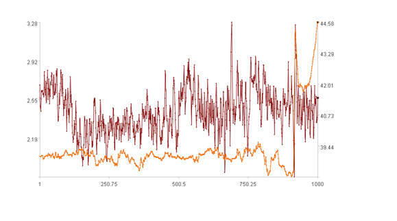
The first figure displays the trends of two time series, with the x-axis representing the sequence index, the left y-axis representing the values of the first dimension, and the right y-axis representing the values of the second dimension. The bold point represents the value of the (k+1)-th point (k=999).
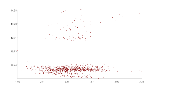
The second figure displays the scatter plots of two time series, with the x-axis representing the values of the first dimension, and the y-axis representing the values of the second dimension. The bold point represents the (k+1)-th point.
The second figure shows that the (k+1)-th point is an outlier, which exactly matches the calculated anomaly score of 0.93.
SPL Official Website 👉 https://www.esproc.com
SPL Feedback and Help 👉 https://www.reddit.com/r/esProcSPL
SPL Learning Material 👉 https://c.esproc.com
SPL Source Code and Package 👉 https://github.com/SPLWare/esProc
Discord 👉 https://discord.gg/sxd59A8F2W
Youtube 👉 https://www.youtube.com/@esProc_SPL

