In industrial production, it’s common to have two or more instruments working together, such as temperature and pressure sensors, or valve opening and flow rate meters. The sequence formed by multiple time series is called a multidimensional time series and is represented by the matrix X.

X is an m-dimensional time series, where its i-th row contains the values of the m time series at the i-th time point, denoted as Xr_i.

Xr_i=[x_i1,x_i2,…,x_im],i∈[1,n]

X consists of the values Xr_i at n time points.

The j-th column of X is the j-th single-dimensional time series, denoted as Xc_j.

X consists of the m single-dimensional time series Xc_j.

X=[Xc₁,Xc₂,…,Xc_m]

Multidimensional time series anomaly detection can follow the same principles and methods as single-dimensional anomaly detection. The underlying principle remains that data that has not occurred or rarely occurs is considered anomalous, and we continue to employ unsupervised learning methods. The key difference is expanding the scope from observing single sequences to multiple sequences, with each row of the multidimensional time series X being regarded as a sample, akin to a point in multidimensional space. Geometrically, anomaly detection expands from single-dimensional space to multidimensional space, but the underlying principle remains the same as in the single-dimensional case: examine whether the current time point data Xr_i is rare compared to a previous interval Xr[-k]_i. We learn a pattern E(…) from Xr[-k]_i to determine whether Xr_i is rare, using the return value of E(Xr_i) to assess the rarity of Xr_i.

Theoretically, there are infinitely many functions for the pattern E(…). Here, we will present common methods for detecting anomalies in multidimensional time series, aiming to spark further discussion.

Each time point in the m-dimensional time series X is a point in m-dimensional space. Points clustered together in some way can be considered frequently occurring points, while points scattered in space are deemed infrequent points, that is, outliers.

For a more intuitive illustration, let’s consider a 2-dimensional case, plotting the time series trend graphs and the scatter plot.

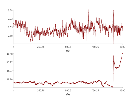
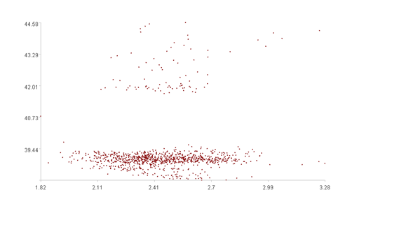
The upper figure displays trend graphs for each of the two time series (the x-axis represents the position index, and the y-axis represents the value).

The lower figure is a scatter plot of the two time series in two-dimensional space (the x-axis represents the value of time series 1, and the y-axis represents the value of time series 2).

It is difficult to discern any patterns from the upper figure. However, the lower figure clearly shows that most points are clustered together, while a few are scattered in space. The goal is to find a pattern E(…) to identify these scattered points.

Clustered points have many “neighboring” points, whereas scattered points have fewer. By counting the number of “neighboring” points for each point and setting a threshold, we can classify data. If the number of neighboring points exceeds the threshold, we consider the data normal and assign an anomaly score of 0. Conversely, if the number of neighboring points is below the threshold, the data is deemed anomalous, with the anomaly score proportional to the deviation from the threshold.

For example, E(…) can be a function such as TA[a₁,a₂,…](…):

TA[S,R](xr_i)=if(N≥S,0,(S-N)/S)

Where S is the threshold for the number of “neighboring” points, R is the radius of the neighborhood, and N is the number of “neighboring” points of the current point Xr_i. S and N are calculated based on Xr[-(k+1)]_i+1 and R.