7.1 Sales trend analysis

Compute sales amount in each month based on historical sales data, find seasonal factor, get deseasonalized sales data, perform linear fitting, and predict sales amount in a specified one of the future months.

Step 1: Retrieve data and compute monthly sales amount.

	A
1	=file(“sales.csv”).import@tc(orderDate,quantity,price,discount)
2	=A1.groups(month@y(orderDate):YMonth;sum(quantity*price*discount):Amount)

A2 In month@y(orderDate), @y option means returning date data of yyyyMM format.

Step 2: Compute average of all the monthly sales amounts.

	A
3	=A2.avg(Amount)

Step 3: Compute seasonal factor.

	A
4	=A2.groups(YMonth%100:Month;avg(Amount)/A3:seasonal_factor).keys@i(Month)

A4 YMonth%100 is the remainder of dividing YMonth by 100 and an integer of MM format is returned. According to such month data, we can compute average sales amount in January, February…. And then divide A3 (the average sales amount of all months) by average of the current month to get the seasonal factor of the current month.

keys@i(Month) sets Month field as both the primary key field and indexed field for the current table sequence, making it convenient to find the seasonal factor by month in a higher efficiency. @i option means setting the indexed field at the same time. When this option is absent, the function only sets the primary key field.

Step 4: Compute desesonalized monthly sales amount.

	A
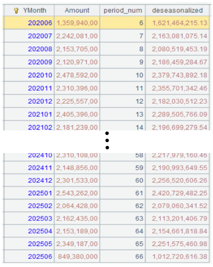
5	=A2.derive((YMonth\100-2020)*12+ YMonth%100:period_num,Amount/A4.find(YMonth%100).seasonal_factor:deseasonalized)

A5 (YMonth\100-2020)*12+ YMonth%100 means gets a natural number sequence whose members are months and use it as the horizontal axis.

The meaning of expression Amount/A4.find(YMonth%100).seasonal_factor: divide the current month’s sales amount by the current month’s seasonal factor and take the retuned value as the deseasonalized sales amount. A4.find(YMonth%100) queries records corresponding to YMonth%100 from A4’s table sequence according to the primary key values. To do this, primary key and indexed field must be created for the table sequence in advance.

Below is result of executing A5’s statement:

Step 5: Perform linear fitting.

	A
6	=linefit(A5.(period_num),A5.(deseasonalized))

A6 Use linear fitting function linefit()to perform linear fitting on the number sequence obtained in A5 and the corresponding deseosonalized monthly sales amount. Here both parameters are one-dimensional vectors. Their corresponding equation is y=ax. In the linefit() function, the first parameter is x, the second parameter is y and the returned value is a, x’s coefficient.

Step 6: Predict the future monthly sales amount.

	A
7	=A6*67
8	=A7*A4.find(67%12).seasonal_factor

A7 According to the above A5’s result, data recording stops at period_num 66, so it is the sales amount of month numbered 67 that we will predict. A6*67 gets the deseasonalized sales amount in month 67.

A8 Multiply A7’s deseasonalized sales amount by the corresponding seasonal factor to get the actual sales amount in month 67.

Learning point: linefit() function

Linear Fitting is an analytical method that uses a linear model (usually a straight line) to virtually represent the relationship between variables in a dataset. It assumes that there is a linear relationship between the dependent variable (target variable) and one or more independent variables (feature variables) and finds the linear equation of the best fit.

Core concepts

1. Linear model:

   • Univariate linear fitting (univariate): Formed asy=ax+b, where:

     • y is the dependent variable
     • x is the independent variable
     • a is the slope (regression coefficient)
     • b is the intercept

   • Multivariate linear fitting (multivariate): Formed asy=a₁x₁+a₂x₂+⋯+b, which is suitable for handling scenarios involving multiple independent variables.

2. Target:

   • Find values of the parameters (slope and intercept) to achieve the minimum error between the model’s prediction value and the actual data point (usually using the Least Squares Method).

3. The Least Squares Method:

   • Find the best fit line by minimizing the residual sum of squares (sum of squares of the differences between the predicted values and the actual values).

Function syntax

linefit(A,Y) Use the least squares method to perform the linear fitting, where the coefficient matrix is A and the constant is Y.

@1 When Y is a vector, the function returns a vector instead of a matrix.

Application scenarios

• Predict the relationship between housing price and room size.
• Analyze the relationship between advertising investment and sales.
• Analyze the trend of experimental data.

Advantages & disadvantages

• Advantages: Simple, efficient, and easy to interpret.
• Disadvantages: Prone to be influenced by anomalies and the effect of non-linear relationship fitting is not good.

7.2 Sales trend analysis

In the preceding example, the analysis only involves months and sales amounts. But in real-world business scenarios, sales amount is closely correlated to the product price and is also influenced by the coefficient, which is intercept b in equation y=ax+b in the preceding example. In this section, let’s look at the relationship between sales amount and the month and product price. The corresponding equation is y=a₁x₁+a₂x₂+b, where x₁ represents the month and x₂ represents product price.

	A
1	=file(“sales.csv”).import@tc(orderDate,quantity,price,discount)
2	=A1.groups(month@y(orderDate):YMonth,price;sum(quantity*price*discount):Amount)
3	=A2.avg(Amount)
4	=A2.groups(YMonth%100:Month,price;avg(Amount)/A3:seasonal_factor).keys@i(Month,price)
5	=A2.derive((YMonth\100-2020)*12+ YMonth%100:period_num, Amount/A4.find(YMonth%100,A2.price).seasonal_factor:deseasonalized)
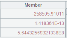
6	=linefit@1(transpose([A5.(period_num),A5.(price),A5.(1)]),A5.(deseasonalized))
7	=file(“product.csv”).import@tc(productID,listPrice)
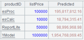
8	=A7.derive((67*A6(1)+listPrice*A6(2)+A6(3))*A4.find(67%12,listPrice).seasonal_factor:Predicted)

In both A2 and A4, price field appears in grouping & aggregation function. And in A4, it is also one of the primary key fields on which the index will be created.

A6 linefit() function works with @1 option to return a sequence instead of a matrix. Parameter transpose([A5.(period_num),A5.(price),A5.(1)]) specifies a matrix made up of three sequences – period_num, price, and sequence 1, where the sequence 1 means intercept b*1.

Below is result of executing A6’s statement:

A7 Import productID field and listPrice field from the product table.

A8 Predict sales amounts of products with different prices in the next month (the month numbered 67). The formula is y=a₁x₁+a₂x₂+b, where a₁, a₂ and b respectively correspond to the three values returned by A6. x₁ is the month number and x₂ is the listed product price.

Below is result of executing A8’s statement:

7.3 Correlation analysis between sales quantity and discount

Does sales quantity is corelated to the discount? Is the bigger the order the greater the discount? Analyzing correlation between them will answer the questions:

	A
1	=file(“sales.csv”).import@ct(quantity,discount)
2	=pearson (A1.(discount),A1.(quantity))

A2 Compute the Pearson correlation coefficient between discount and sales quantity.

Learning point: pearson() function

Pearson correlation coefficient (represented by r) is a statistic that measures the strength and direction of linear correlation between two continuous variables. The range of its values is [−1,1].

Core concepts

1. Definition:
   • It measures the linear correlation between two variables X and Y.
   • The formula of computing Pearson correlation coefficient:

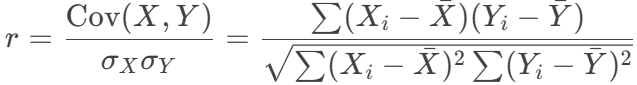
Where:

• Cov(X,Y) is covariance
• σX,σY is standard deviation
• are means

2. Value range:

• r=1: Perfect positive correlation (The variables show a strictly increasing linear relationship).
• r=−1: Perfect negative correlation (The variables show a strictly decreasing linear relationship).
• r=0: Non-linear correlation (but possibly with a non-linear relationship).

3. Characteristics:

• Only suitable for handling linear relationships but cannot catch a non-linear correlation (such asy=x2y=x2).
• Sensitive to anomalies; extreme values may noticeably influencethe value of r.
• Within the value range [−1,1], the larger the absolute value, the stronger correlation.

Function syntax

pearson(A,B) Compute Pearson correlation coefficient between variable A and variable B. Use to(*A.*len()) when parameter B is absent.

@r Compute r²; this is equivalent to pearson(norm@0(A),norm@0(B)).

@a(…;k) Compute the adjusted r², with degrees of freedom being k.

How to interpret Pearson correlation coefficient?

Value range of r			Degree of correlation
0.8<	r	< 1	Strong correlation
0.5<	r	< 0.8	Moderate correlation
0.3<	r	< 0.5	Weak correlation
0 <	r	< 0.3	Extremely weak or no correlation

7.4 Analysis of mean differences in product sales quantity

To find if there is a big difference between esProc average sales quantity and the other products’ average sales quantity, you can use the t-test:

	A
1	=file(“sales.csv”).import@tc(product,quantity)
2	=ttest_p(A1.(if(product==“esProc”:0;1)),A1.(quantity))

A2 In SPL, ttest_p() function performs t-test. The input parameters are two sets of sequences. One is a binary sequence made up of 0 and 1; the other is a sequence consisting of numbers to be analyzed. The function automatically splits the second sequence into two sets of numbers corresponding to 0 and 1 respectively and compare them.

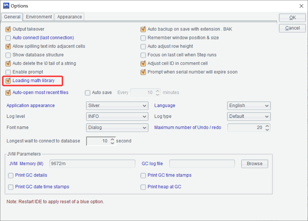
ttest_p() is an external library function. You need to first load the external library to use it according to the following directions:
1、 Click Tool/Options
2、 Check Loading math library

Learning point: ttest_p() function

t-test is a statistical hypothesis test used to determine if there is a significantly difference between the means of two sets of data. It is based on t-distribution (Student’s t-distribution) and suitable for handling scenarios where the sample size is not large (usually n<30) and the population variance is unknown.

Core concepts

• Target: Compare means of two sets of data to determine whether the difference is due to random errors or is statistically significant.
• Requirements:
  • Data should be nearly normal distribution (or the sample size should be large enough to depend on the Central Limit Theorem).
  • Homogeneity of variance (Some t-tests require that between-group variances are equivalent).

• Output:

  • p-value: If p<0.05 (usually of significance level), the result is considered statistically significant.

Function syntax

ttest_p(X, Y) Perform t-test to find the p-value.

Application scenarios

• Compare whether there is a significant difference between click-through rates among two groups of users in A/B tests.
• Compare difference of same sample in different conditions (such as blood pressure changes before and after taking the medicine).
• Check if there is a significant change in body weight of trainees before and after weight loss training.

To find differences between means of sales quantities of all products, you can use ANOVA test. The corresponding method in SPL is fisher_p() function:

	A
1	=file(“sales.csv”).import@tc(product,quantity)
2	=fisher_p(A1.(product),A1.(quantity))

A2 fisher_p() function is used to compare means of multiple sets of data. It does not split data into groups; instead, it gets the sequence of grouping field values and the sequence of numeric values directly and splits the numeric values into multiple groups automatically according to the grouping field values for comparisons.

Learning point: fisher_p() function

fisher_p() function uses ANOVA (Analysis of Variance) test, which is a statistical method for finding whether there is a significant difference between means of three or more sets of data. Its core idea is to analyze the data’s variance (variability) to find if the inter-group difference is significantly greater than the intra-group difference.

Core concepts

(1) Why use ANOVA?

• Limitations of t-test: t-test can only compare means of two sets of data. When comparing means of more sets of data, the pairwise comparisons will increase the probability of Type I error (false positive).
• Advantages of ANOVA: Find difference of means of multiple sets of data at one time and control the overall error rate.

(2) Basic hypothesis

• Normality: Each set of data should be nearly normal distribution (or the sample size should be large enough).
• Homogeneity of Variance: Variances of the sets of data should be similar (can be checked through Levene’s test).
• Independence: Observed values are independent from each other (for example, samples of different groups are unassociated).

(3) Hypothesis testing

• Null hypothesis (H₀): Means of all groups are equal (μ₁ = μ₂ = … = μₖ).
• Alternative hypothesis (H₁): Means of at least two groups are unequal.

Function syntax

fisher_p(X, Y) Perform F-test to find the p-value.

ANOVA vs T-test

Item	ANOVA	T-test
Number of to-be-compared groups	≥3 groups	2 groups
Application scenario	Difference of means of 3 or more groups	Difference of means of 2 groups
Post-hoc analysis	Needed	Directly interpret the result
Statistical value	F-value	t-value

4. Result interpretation

• p-value:
  • If p<0.05, reject H₀ and consider that means of at least two groups are different.
  • If ANOVA is significant, post-hoc test is needed to determine the specific differences between groups.

7.5 RFM analysis on customer transaction data

RFM analysis (recency of purchase, frequency of purchases, Monetary value) assesses customer purchase behaviors. Define a custom function, which receives three input parameters – transaction data and referenced date. The most recent purchase time (R) represents the number of days since last purchase, which is the smaller the better. The frequency of purchases (F) represents the total number of purchases, which is the larger the higher frequency of the purchase. The monetary value (M) is the total expenditure amount, which is the larger the higher-value the customer is. To make the dimension consistent, each sub-dimension will be sorted and their values are converted to standard scores between 0 and 5 – sort the latest purchase time points in descending order (as recent purchases are more ideal) and purchase frequences and purchase amounts in ascending order (as more purchases and higher amounts are more desirable).

	A	B
1	=file(“sales.csv”).import@ct(customer,orderDate,quantity,price,discount)
2	func rfm_score(data,current_date)
3		=data.groups(customer; interval(max(orderDate),current_date):recency, count(1):frequency, sum(quantity*price*discount):monetary)
4		=B3.len()
5		=B3.derive(:r_score,: f_score,:m_score)
6		=B5.sort(recency:-1).run(r_score=rank(recency)/B4*5)
7		=B5.sort(frequency).run(f_score=rank(frequency)/B4*5)
8		=B5.sort(monetary).run(m_score=rank(monetary)/B4*5)
9		return B5
10	=rfm_score(A1,now())

A1 Import data from sales.csv.

A2 Define a function named rfm_score and having parameters data and current_date.

B3 Group input parameter data by customer and compute the number of days between the latest purchase time and the referenced date, the number of purchases, and the total purchase amount.

B4 Get the total number of records in B3.

B5 Add three new fields – r_score, f_score and m_score.

B6-B8 Compute values for r_score, f_score, m_score fields respectively. Expression rank(recency)/B4*5 computes rankings according to recency, divides the ranking by the total number of records to get the ranking percentage, multiplies the percentile by 5, and returns a value that falls within 0~5. Use a similar way to compute values for the other two fields, only with an opposite sorting direction.

B9 Return the result.

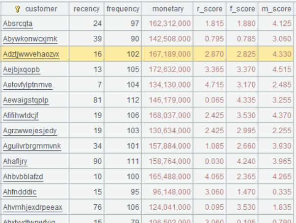
A10 Call custom function rfm_score and pass parameters A1 and now() to it.

Below is result of executing A10’s statement:

Learning point: What is a code block?

The following shows one:

A2 is a non-null cell, which commands a cell range, where A3:A9 are blank cells and A10 is non-null. In this case, cell range B3:B9 is a code block with A2 being its master cell.

Core characteristics of the code block

1. Indent-sensitive:

• Cells in the same indent belong to the same code block.
• A blank cell is usually used as the indent unit.

2. Code block rules:

• A variable defined in a code block is invalid only within the block.
• A code block can access outside variables.

3. Process control:

• A code block is made up of a branch and a loop statement in the indent form.

Main application scenarios

1. Function definition

	A	B	C
1	=func factorial(n)
2		if n==1
3			return 1
4		else
5			return n*factorial(n-1)

2. Conditional statement

	A	B
1	=x=10
2	if x>5
3		=“>5”
4	else
5		=“<=5”

3. Loop structure

	A	B
1	=i=1
2	for i<=5
3		>output=output+" "+string(i)
4		>i=i+1

4. Exception handling

	A	B
1	try
2		=1/0
3	if A1!=null
4		=“error”
5	else
6		=“correct”

Multilevel code block

	A	B	C	D
1	=func process(data)
2		=result=[]
3		for data
4			if #B3%2==0
5				=result.insert(0,B3)
6		return result

Characteristics of code block execution

• Independent execution environment: Each code block has its independent variable scope.
• Return value: Return value of the last expression as the final value of the code block.
• Cell coordination reference: Reference a value in another code block using the cell coordinate (such as A1).

Differences from Excel formulas

• Structured programming: Support true code blocks and process control.
• Variable scope: More flexible cell reference than Excel’s.
• Function features: Support advanced function features, such as recursion and higher-order functions.

esProc SPL’s code blocks feature a cell range and indents. Not only are they, like Excel, intuitive, but they provide all-round programming abilities, making them particularly suitable for dealing with complicated data computing tasks.

Learning point: Custom functions

Basic syntax

	A	B
1	=func funcName(arg1,arg2,……)
2		Indented Function Block

Complete examples of function definitions

1. Basic functions

	A	B
1	=func add(a,b)
2		=a+b
3		return B2
4	=add(3,5)

A1 Define a function.

B2 Function body (Indent text by one cell)

B3 Return value (this statement can be omitted; by default, return value of the last expression).

A4 Call the function and return 8.

2. Functions with default parameters

	A	B
1	=func greet(name=“Guest”,greeting=“Hello”)
2		=greeting+“,”+name+“!”
3		return B2
4	=greet()
5	=greet(“John”)
6	=greet(“Mary”,“Hi”)

A4 Return “Hello, Guest!”

A5 Return “Hello, John!”

A6 Return “Hi, Mary!”

Characteristics of function code block

1. Indentation rules:

• After function declaration each cell with the same number of indented cells before it is a part of the function body.
• Usually, the standard indentation is one empty cell.

2. Scope control:

• Separate local variables from outside variables.
• Allow accessing global variables outside (but be careful to do this).

3. Multi-statement execution:

• A function body may contain multiple statements that will be executed sequentially.

7.6 Categorizing customers into five groups based on RFM analysis result

According to the RFM analysis result in the preceding example, categorize customers into five groups using two methods. One method is to perform the grouping according to the three types of scores: r_score, f_score, m_score; the other is to do this according to the weighted scores.

Method 1:

	A
…	// Continue from the preceding example
11	=kmeans(A10.([r_score,f_score,m_score]),5)
12	=kmeans(A11,A10.([r_score,f_score,m_score]))

A11 According to scores r_score, f_score, m_score, categorize customers into five groups using clustering method K-means. In SPL, kmeans() function uses the classic unsupervised learning clustering algorithm, which will be illustrated in subsequent sections.

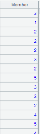
A12 Return the ID of category to which each customer belongs according to A11’s clustering result. Customers having the same category ID belong to the same category.

Below is result of executing A12’s statement:

Method 2: Weight the three types of scores – the purchase amount is the most important and is given 3 in weight; the purchase frequency is of secondary importance and is given 2 in weight; the most recent purchase date is weighted as 1, and group customers anew according to the weighted scores:

	A
…	// Continue from the preceding example
11	=kmeans(A10.([r_score,f_score*2,m_score*3]),5)
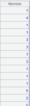
12	=kmeans(A11,A10.([r_score,f_score*2,m_score*3]))

Below is result of executing A12’s statement:

Learning point: kmeans() function

Kmeans algorithm description:

K-means is a classic unsupervised learning clustering algorithm. It divides a data set into K clusters. The data points in one cluster have greater similarity than data points in different clusters.

Syntax of kmeans() function

kmeans(X, k ) Use k-means clustering algorithm to divide matrix X into k clusters and return fit model B.

kmeans(B, A ) Use k-means clustering algorithm to analyze data set A** according to fit model B and return the cluster number to which A belongs.

Steps of performing the k-means algorithm

1. Initialization: Randomly choose K data points and make them the initial centroids.
2. Assignment step: Assign each data point to the cluster whose centroid is closest to it.
3. Update step: Recompute the centroid of each cluster (the mean of all data points assigned to the cluster).
4. Repeat: Repeat step 2 and step 3 until the centroids no longer change significantly or the maximum number of iterations is reached.

Application scenarios of k-means algorithm

1. Customer segmentation

• Divide customers into different groups based on characteristics such as purchase behaviors and demographics.
• For precision marketing and personalized recommendations.

2. Image compression

• Reduce the number of image colors to K representative colors.
• Reduce storage usage while maintaining quality visual effect.

3. Document classification

• Perform clustering on text documents.
• Locate topic groups in a set of documents.

4. Anomaly detection

• Identify anomalies far from any cluster centers.
• For fraud detection, network intrusion detection, etc.

5. Market segmentation

• Market segmentation based on geography and consumption habits.
• Help draw up regional marketing strategies.

Advantages and disadvantages of k-means() function

Advantages:

• Simple, easy to understand and implement.
• Highly efficient and thus suitable for handling large data sets.
• Good performance in handling spherical cluster data.

Disadvantages:

• Need to specify K-value in advance.
• Sensitive to the choice of initial centroid.
• Sensitive to noises and anomalies.
• Can only identify spherical clusters and is difficult to handle clusters having complex shapes.imagepng