5.1 Data information

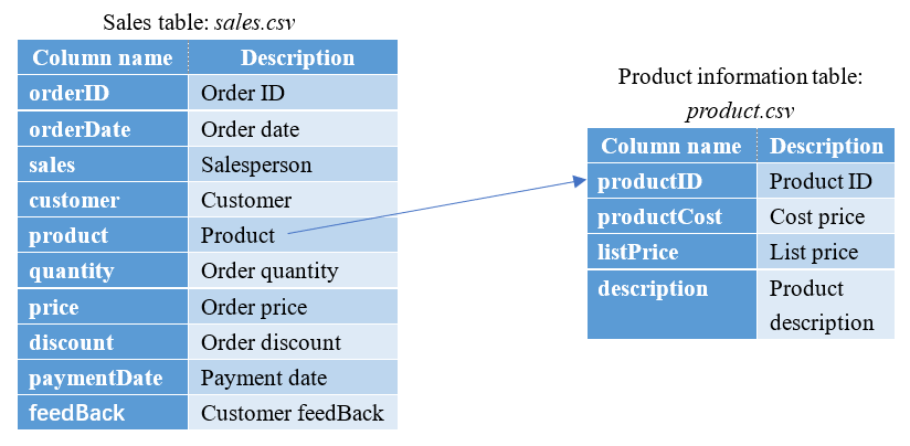
Here is product information table product.csv. It consists of fields shown below:

Column name	Description
productID	Product ID
productCost	Cost price
listPrice	List price
description	Product description

Relationship between product.csv and the above-mentioned sales table sales.csv:

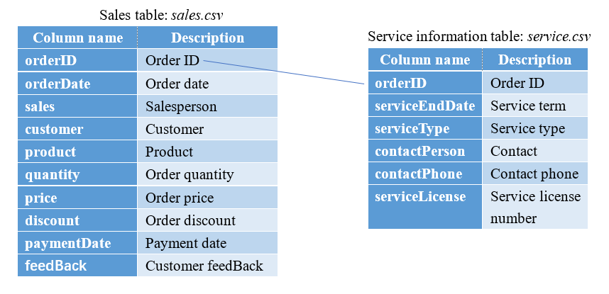
Here is service information table product.csv. It consists of fields shown below:

Column name	Description
orderID	Order ID
serviceEndDate	Service term
serviceType	Service type
contactPerson	Contact
contactPhone	Contact phone
serviceLicense	Service license number

Relationship between service.csv and the above-mentioned sales table sales.csv:

5.2 Compute total sales of each product per month (grouping & aggregation)

We can use the above-mentioned grouping operation to compute total sales of each product per month:

	A
1	=file(“sales.csv”).import@tc(paymentDate,product,quantity,price,discount)
2	=A1.select(paymentDate)
3	=A2.groups(month@y(paymentDate):Month,product;sum(quantitypricediscount):Amount)

A1 Read to-be-used fields from sales.csv. Since the aggregation is on sales amounts, it is more reasonable to sum amounts according to the actual payment dates. That’s why the date field retrieved is paymentDate instead of orderDate.

A2 Select records where paymentDate isn’t null. Here paymentDate is equivalent to paymentDate!=null; it is the latter’s simplified form.

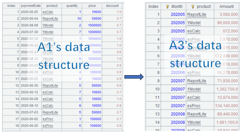
A3 Group records by month and product and compute total sales in each group. In month@y(paymentDate), @y option enables returning an integer of yyyyMM format. When this option is absent, the function returns MM only.

Grouping and aggregation is the most commonly seen operation that results in change of data structure:

5.3 Compute MoM rate by product (pivot aggregation)

Convert A3’s data to the following format:

Month	esProc	esCalc	ReportLite	YModel
202005				.
202006				.
202007				.
……				.

And then compute MoM rate by product:

Month	esProc	Proc_MoM	esCalc	Calc_MoM	ReportLite	Report_MoM	YModel	YM_MoM
202005			…					.
202006								.
202007								.
……								.

Step 1: Pivot computation

	A
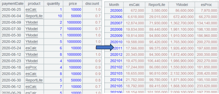
4	=A3.pivot(Month;product,Amount)

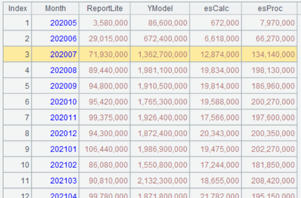
A4 Perform pivot computation on A3’s data. The 1^st parameter Month means performing grouping on the leftmost column by Month. The 2^nd parameter product means making product field values the column headers; the number of to-be-generated columns is determined by the number of unique product values. The 3^rd parameter Amount means the intersection is Amount field value. The 1^st parameter and the 2^nd parameter are separated by semicolon, and the 2^nd parameter and the 3^rd parameter are separated by comma.

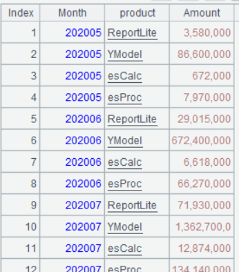
Below is result of executing A4’s statement:

Step 2: Compute MoM rate by product. With the data structure of the preceding step’s pivot computation result, it is easy to get the task done using the previously mentioned [-1] operator to

	A
5	=A4.new(Month,esProc,(esProc-esProc[-1])/esProc[-1]:Proc_MoM,esCalc,(esCalc-esCalc[-1])/esCalc[-1]:Calc_MoM,ReportLite,(ReportLite-ReportLite[-1])/ReportLite[-1]:Report_MoM,YModel,(YModel-YModel[-1])/YModel[-1]:YM_MoM)

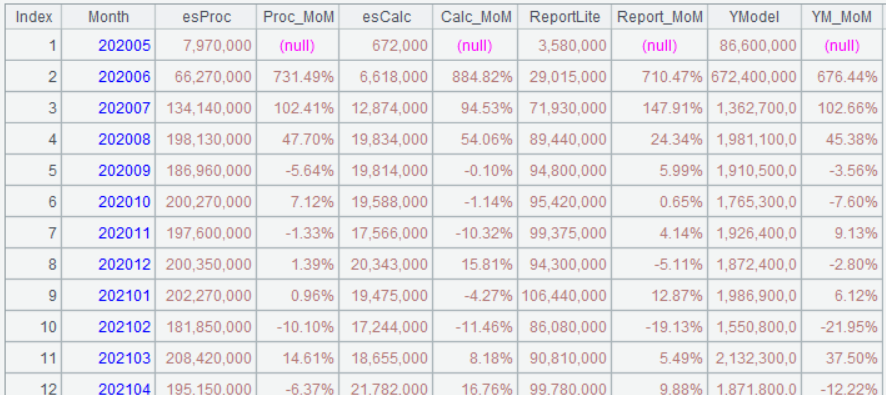
Below is result of executing A5’s statement:

To change pivot-sectional data back to group format data, pivot@r is used. For example, to convert A4’s result back to A3’s format, the following statement is used:

	A
6	=A4.pivot@r(Month;product,Amount)

Below is result of executing A6’s statement:

Learning point: pivot() function

esProc SPL’s pivot() function is powerful in handling data pivoting. It transforms rows/columns of a table sequence/record sequence to columns/rows. The effect is basically amounts to Excel PivotTable.

Syntax:

$$
A.pivot(g:G , … ; F, V; Ni:N’i,…)
$$

Parameter:

A	A table sequence/record sequence.
g	Grouping field/grouping expression.
G	Field name in the result set; default is g.
F	A field name in A.
V	A field name in A.
Ni	F field values, which can be omitted. By default, they are all unique values of F field.
N’i	Names of new fields, which, by default, are Ni.

Option:

@r	Perform column-to-row transposition on a table sequence/record sequence. Field names Ni will become values of F field after transposition; when parameter N’i is present, it will replace Ni to become F field values, and values of the original Ni fields will become values of new field V. Default values of Ni are all field names in A except for g,….
@s(g:G,…;F,f(V);Ni:N’i,…)	f can be an aggregate function, including sum, count, max, min and avg. It can be written as ~.f(), where ~ references the current group. When N’i is present and Ni is absent, perform aggregation on field V whose values have not been summarized when they are under Ni field.

Return value:

Table sequence

Function diagram:

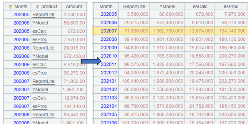
A3.pivot(Month;product,Amount)

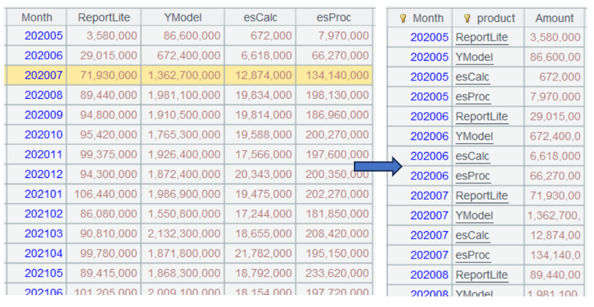
A4.pivot@r(Month;product,Amount)

A2.pivot@s(month@y(paymentDate):Month;product,sum(quantitypricediscount)) is equivalent to the combination of A3 and A4. It combines grouping & aggregation and pivot computation in one expression.

5.4 Gross profit tracking (foreign key-based join)

A salesperson’s monthly gross profit target is 1000000. We want to select orders in October in 2024 and track daily cumulative gross profit completion rate.

Formula for computing gross profit: product’s actual sales price – cost price.

Step 1: Create association between sales data table and product information table

The product’s cost price is stored in product information table, but the actual sales price is stored in sales data table. To compute gross profit, first we need to create association between two tables:

	A
1	=file(“product.csv”).import@tc(productID,productCost)
2	=file(“sales.csv”).import@tc(paymentDate,product,quantity,price,discount)
3	=A2.select(month@y(paymentDate)==202410).sort(paymentDate)
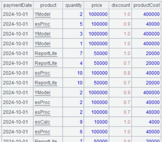
4	=A3.join(product,A1:productID,productCost)

A4 A3.join(product,A1:productID,productCost) creates association between A3 and A1 through A3’s product field and A1’s productid field, which are join fields, and then adds A1’s productCost field to A3. Note that A1 and productID are separated by colon, which means productid is one of A1’s fields.

Below is result of executing A4’s statement:

Step 2: Group records by date and compute gross profit in each group.

	A
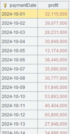
5	=A4.groups(paymentDate;sum(quantity*(price*discount-productCost)):profit)

A5 Expression quantity*(price*discount-productCost) can be directly written in the sum() function without explicitly adding a computed column.

Below is result of executing A5’s statement:

Step 3: Compute cumulative gross profit.

	A
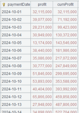
6	=A5.derive(cum(profit):cumProfit)

A6 cum()is a cumulative sum function. cum(profit) is equivalent to the previously mentioned cumProfit[-1]+profit.

Below is result of executing A6’s statement:

Learning point: What is a foreign key-pointed dimension table?

A foreign key-pointed dimension table is a dimension table stored in the relational database. It is associated with the fact table through its foreign key and used for storing descriptive, categorical or reference data. Such a table usually contains static or slowly changing data (such as product, customer and region information), while a fact table stores quantitative business data (such sales amount and order quantity). The major role of a foreign key-pointed dimension table is to provide necessary context information queries and analyses will use, giving fact table higher business significance.

Diagram: Relationship between foreign key-pointed dimension table and fact table:

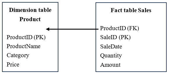
• Dimension table (Product): Store detailed product information (such as product name, type and price), where ProductID is the primary key (PK).
• Fact table (Sales): Store sales transaction data (such as sales date, quantity and amount), where ProductID is the foreign key (FK), which links to the related dimension table.

Characteristics of foreign key-pointed dimension table:

• Stores descriptive data (such as product name, customer information and region information).
• Usually smaller than the fact table because the latter stores a huge amount of transaction data.
• Used in data analytics (such as OLAP and BI reporting) to provide business data context.
• Has a Slowly Changing Dimension (SCD), such as customer addresses.

Summary

A foreign key-pointed dimension table associates with the fact table via the foreign key, providing readable descriptive information for numeric business data (such as sales amount and order quantity). It is one of the core parts in both data warehousing analysis and commercial BI analysis.

5.5 Query information of active customers (one-to-one primary key-based join)

Select information of active customers, including customer name, product name, service end date, service license number.

Step 1: Perform filtering on service table service.csv

As one order may correspond to multiple service tickets, first we order the service tickets by order ID and service end date, select service tickets having the latest end date and then those still within the service period. In this case the records to be involved in the association will be fewer and efficiency will be increased.

	A
1	=file(“service.csv”).import@tc(orderID,serviceEndDate,serviceLicense)
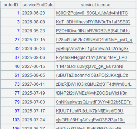
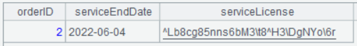
2	=A1.sort(orderID,-serviceEndDate).group@o1(orderID).select(serviceEndDate>now())

Below is result of executing A2’s statement:

Step 2: Create association between A2 and sales data table sales.csv and get corresponding customer names and product names.

According to the information about sales.csv introduced previously, orderID values are a natural number series, which correspond to record numbers. So, we can perform the join through the correspondence between A3’s record numbers and A2’s orderID field values.

	A
3	=file(“sales.csv”).import@tc(orderID,customer,product)
4	=A2.join(orderID,A3:#,customer,product)

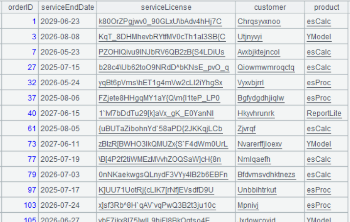
A4 Perform join between A2 and A3 via join fields, which are A2’s orderID field and A3’s record numbers respectively (in a loop function, # represents ordinal number of the current record), and add corresponding customer and product fields of A3 to A2.

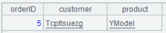
Below is result of executing A4’s statement:

Learning point: What is #?

In SPL, # is the built-in system variable representing the sequence number (integer ordinal numbers starting from 1) of the current record in a sequence. The symbol plays a fundamental role in iterative computation, record location and table sequence handling by providing a concise reference method for performing operations related to data traversal and position determination. The record sequence number # has some key characteristics:

1. Auto-generated: It is a sequence of continuous integers automatically generated by the system.
2. Read-only: Cannot modified through assignment.
3. Dynamically changing context: Automatically updated in each iteration.
4. Stably ordered: Always reflect the physical storage order of the original sequence.

Technical characteristics:

Characteristic	Description
Value range	From 1 to the total record count in a table sequence.
Reference context	All computing contexts involving position determination, such as derive(), new(), run().
Special value	Null will be returned when the access exceeds the head and tail boundaries of a table sequence.
Combination use	Often work with ~ (symbol of referencing the current member). For example, ~.# means the sequence number of the current record.

Typical application scenario examples

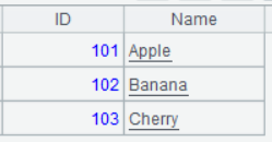
1. Create an example table sequence

	A
1	=create(ID,Name).record([101,“Apple”],[102,“Banana”],[103,“Cherry”])

2. Display record sequence number and record content

	A
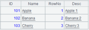
2	=A1.derive(#:RowNo, Name+“:”+string(#):Desc)

3. Perform conditional filtering to select records whose sequence numbers are even numbers.

	A
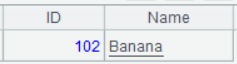
3	=A1.select(#%2==0)

4. Extract records according to record sequence number interval.

	A
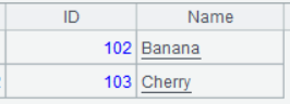
4	=A1.to(2,3)

Below lists some results of executing the above statements:

A1’s result:

A2’s result:

A3’s result:

A4’s result:

Special uses:

• Intra-group reference: During a grouping operation, # begins the count from 1 in each group.
• Working with ~: ~.# is equivalent to the use of # alone. The combination use emphasizes the sequence number property of the current record.
• Performance optimization: The sequence number-based access has O(1) time complexity, which does not affect the computing performance.

The design enables SPL to produce concise code while having direct control on the data order during traversal and position-related computations.

5.6 Service ticket summarization (One-to-many inner join between primary table and subtable)

Select customer name, product name, corresponding number of service tickets, and the latest service end date from each order.

	A
1	=file(“service.csv”).import@tc(orderID,serviceEndDate,serviceLicense)
2	=file(“sales.csv”).import@tc(orderID,customer,product)
3	=join(A2:sales,orderID; A1:service,orderID)
4	=A3.groups(sales.orderID;sales.customer,sales.product,count(1):serviceNum, max(service.serviceEndDate):serviceEndDate)

A3 join() function has similar effect to SQL join. It performs inner join when no options work. The expression in this cell means performing inner join between primary table A2 an subtable A1 through A2’s orderID field and A1’s orderID field, which are the join field. The counterpart SQL code is generally like this:

select sales.*,service.* 
from sales.csv sales
inner join service.csv service on sales.orderID==service.orderID

Below is result of executing A3’s statement:

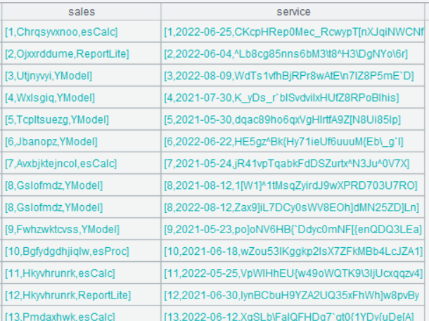
According to the above screenshot, the result set has two fields, which are sales (storing A2’s records) and service (storing A1’s records). Double-click a field value in any row of sales field, we can view the following:

Double-click a field value in any row of service field, we can view the following:

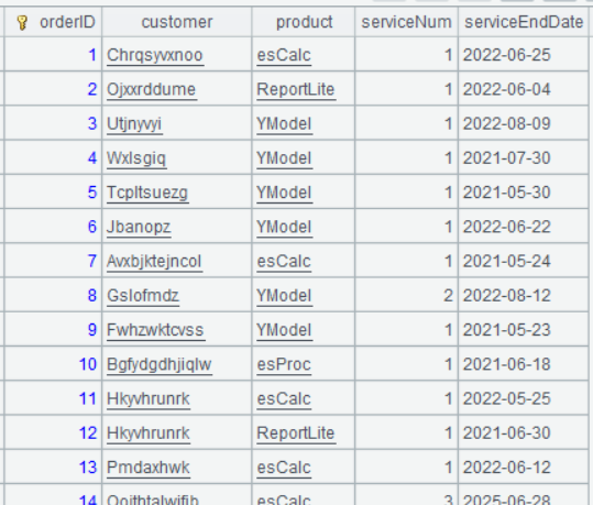
A4 Perform grouping & aggregation on A3. Since both sales field and service field store records, the dot operator (.) can be used to access the field value of a record, such as sales.customer, which accesses customer field value of the record stored in sales field. For fields that don’t take part in the grouping operation but whose values are uniquely determined by the grouping field, thy can be written after the semicolon without an aggregate function, such as sales.customer,sales.product, whose values are determined by orderID and which won’t be grouped. There is no need to write an aggregate function with them.

Below is result of executing A4’s statement:

Learning point: Differences between A.join()and join()

Both functions are used for performing table joins. The main differences between them are these:

Application scenarios:

A.join(C:.,T:K,x:F,…; …;…) is mainly used for performing a join between the fact table and the foreign key-pointed dimension table. A is the fact table and T is the foreign-key pointed dimension table. The join field values in T must be unique, and on most occasions, the field is T’s primary key.

join(Ai:Fi,xj,..;…) is mainly used for performing primary key-based joins. The function works in a similar way to a SQL join. It supports inner join, left join, and full join.

Parameter structure:

In A.join(C:.,T:K,x:F,…; …;…), except for specifying the table to be joined and the join field, the parameter can also specify a field or expression to be appended to A. The parameter structure is more complicated than that in join().

In join(Ai:Fi,xj,..;…), parameters only responsible for specifying the table to be joined and the join field.

Result set:

A.join(C:.,T:K,x:F,…; …;…) directly returns the result set as a table sequence, which can be directly exported or displayed.

join(Ai:Fi,xj,..;…) returns the result set as a referencing field, which needs a further new or groups operation to become the final result for display.

Learning point: What are primary table and subtable?

The primary-subtable structure is a typical database design that represents the one-to-many relationship. It consists of a primary table (Master) and its subtable(s) (Detail). The primary table holds core entity data (information of, such as, orders, students, articles); the subtable(s) stores detailed data (such as products purchased in orders, students’ scores, comments on articles) related to the records of the primary table. Each primary table record corresponds to multiple records in the subtable, but one subtable record must and can only belong to one primary table record. Such a relationship is implemented through foreign key constraint and guarantees data integrity, for example, when a primary table record is deleted all levels of related records in a subtable are deleted synchronously.

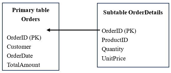
Diagram

Use case

An ecommerce system example:

Primary table Ordersstores main order information (orderID 1001, Customer John, 2023-01-01).

Subtable OrderDetailsholds information of all products in the orders record:

Record 1: OrderID 1001 (related field), Product A, two pieces, unit price ¥50

Record 2: OrderID 1001 (related field), Product B, one piece, unit price ¥200

The structure avoids data redundancy in the primary table (no need to stuff one orders record with all its product information) while completely storing orders details. It is the standard design model in relational databases.

5.7 Get customers placing an order in October and count orders in both October and November (left join)

Step 1: First, respectively select orders records in October and November in 2024.

	A
1	=file(“sales.csv”).import@tc(orderDate,customer)
2	=A1.select(month@y(orderDate)==202410)
3	=A1.select(month@y(orderDate)==202411)

Step 2: Count orders in the two months respectively.

	A
4	=A2.groups(customer;count(1):octNum)
5	=A3.groups(customer;count(1):novNum)

Step 3: Perform left join

	A
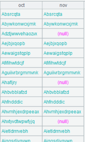
6	=join@1m(A4:oct,customer**;** A5:nov,customer)
7	=A6.new(oct.customer,oct.octNum, nov.novNum)

A6 Perform left join between A4 and A5 though A4’s customer field and A5’s customer field, which are the join field. @1 option, which uses number 1 instead of letter l, means left join. @m option means same-order association. When both A4 and A5 are ordered by the join field, @m option can be used to perform the same-order association. The merge algorithm helps increase efficiency. When @1 option and @m option work together, they can be written as @1m.

Below is result of executing A7’s statement:

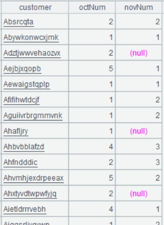
A7 Generate a new table sequence based on A6 – retrieve fields to be exported from the referencing field and export them as the final result.

Below is result of executing A7’s statement:

5.8 Count orders Customers place in October, November, December (full join)

Step 1: Select records of orders placed in October, November and December respectively.

	A
1	=file(“sales.csv”).import@tc(orderDate,customer)
2	=A1.select(month@y(orderDate)==202410)
3	=A1.select(month@y(orderDate)==202411)
4	=A1.select(month@y(orderDate)==202412)

Step 2: Count orders in the three months respectively.

	A
5	=A2.groups(customer;count(1):octNum)
6	=A3.groups(customer;count(1):novNum)
7	=A4.groups(customer;count(1):decNum)

Step 3: Perform full join

	A
8	=join@fm(A5:oct,customer ; A6:nov,customer ; A7:dec,customer)
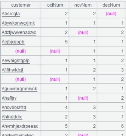
9	=A8.new(oct.customer,oct.octNum, nov.novNum,dec.decNum)

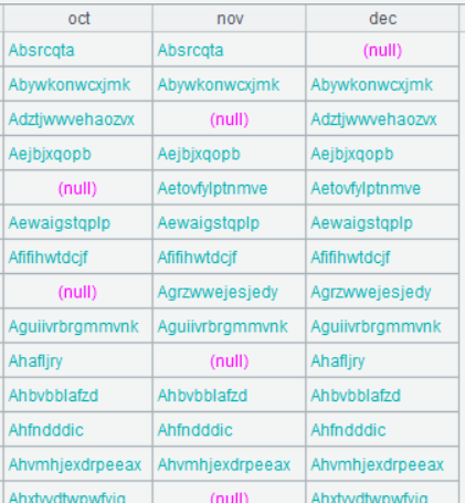
A8 @f means full join.

Below is result of executing A8’s statement:

Below is result of executing A9’s statement: