Data information

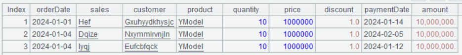
Below is a table (sales.csv) recording a company’s sales data:

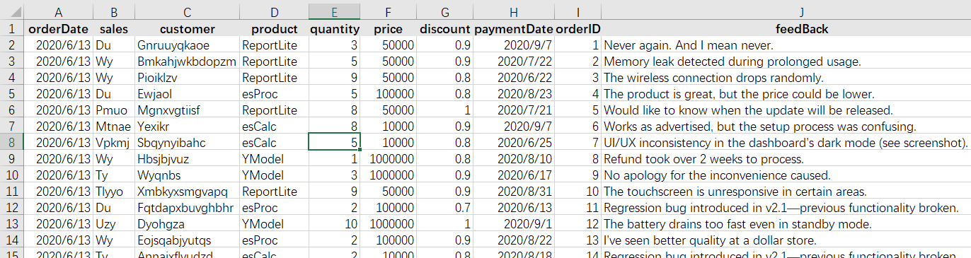
The first row contains headers, describing what each column stores. From the second row, each row forms a record, which corresponds to an order.

There is a special term, structured data, for this type of data. They are the most commonly seen data type in today’s data processing scenarios. The whole table of data is called a data table, where each row (except for the header row) is called a record and where each column is a field. Each string in the header row is a field name. In the visible part of the above spreadsheet, there are 12 records, which correspond to rows from the 2^nd to the 13^th. The table has 8 fields – orderDate, sales, customer, product, quantity, price, discount, paymentDate. These field names are different from each other and can uniquely identify a column. The fields (including their names and order) constitute the table’s data structure, simply called structure.

Structured data is data having a certain structure.

Cell range A2:H13 in the above spreadsheet has all data in the data table. It is common to say that the value of a certain field in a certain record is xxx. In the above table, for example, the 2^nd record’s sales field value is Hef and the 8^th record’s quantity field value is 8. Every field of each record has its value.

Note that in a data table only the field has name; the record does not have a name. In one of the later sections we’ll talk about the method used to identify records and differentiate them from each other.

There are various kinds of data tables. It is normal that different data tables have different structures. A data table must and can only have one structure. Sometimes we talk about the record structure, which also refers to the structure of the data table where the record resides.

As structured data is often displayed in the form of a table made up of rows and columns, records and fields are often intuitively called rows and columns, which is a database tradition rather than a practice invented by SPL. Sometimes even there are not visible rows and columns in a data table when it is displayed (there is such a table in one of the following examples), specialized terms rows and columns are still used to refer to records and fields.

Here are descriptions of column names in sales.csv used in this document:

Column name	Description
orderID	Order ID, whose value range is a sequence of natural numbers, which correspond to the records’ sequence numbers
orderDate	Order date
sales	Salespeople
customer	Customer
product	Product
quantity	Order quantity
price	Order price
discount	Order discount
paymentDate	Payment date
feedBack	Customer feedback

Select all sales records in the last year

Step1: Read data from sales.csv.

	A
1	=file("sales.csv").import@tc()

A1 The file("sales.csv") function finds file sales.csv from the main directory and generates the file object. Its parameter is a string, and so is enclosed by double quotation marks. The import@tc() function reads data from file object file(“sales.csv”); @t is the function’s option, meaning reading the file’s first line as the header row. If this option is absent, the first line will be treated as data to be imported. @c enables using comma as the column separator when importing data from the file; without this option, tab will be used as the column separator by default. When both @t and @c are used, one @ symbol can be omitted and the syntax is simply @tc.

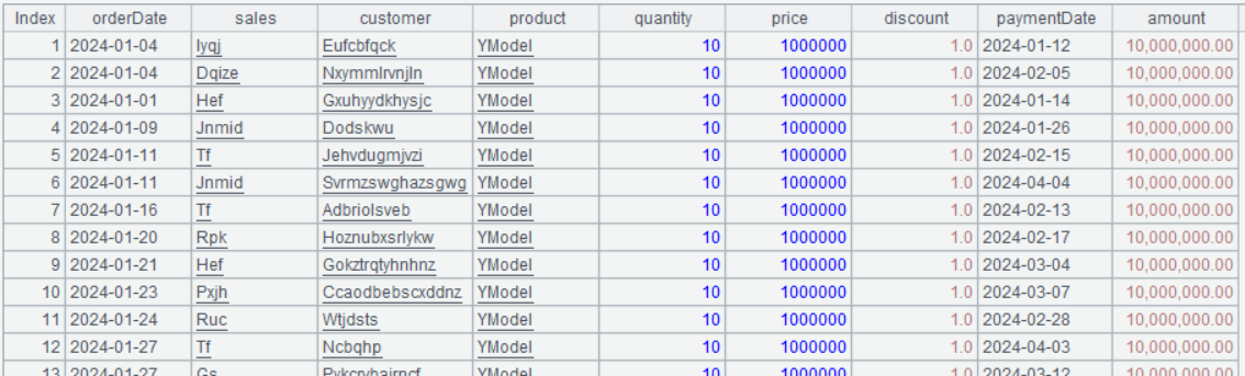
A1’s value can be viewed on the interface:

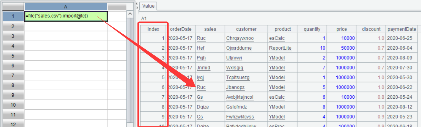
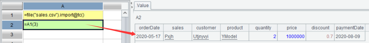
You can see that A1’s value is a two-dimensional table. As mentioned above, sales.csv stores structured data. In SPL, an object that loads and stores structured data is called table sequence, which can be literally understood as an ordered two-dimensional table. In the above screenshot, A1’s value is a table sequence. But compared with the original structured data this table sequence has an Index column, which records the order of records in the table sequence. The Index column values are also called record sequence numbers. According to a sequence number, we can access the corresponding record. Expression =A1(3), for example, returns the 3^rd record in A1:

Step 2: Get records of orders placed in the year 2024 from A1:

	A
1	=file(“sales.csv”).import@tc()
2	=A1.select(year(orderDate)==2024)

A2 The select() function performs filtering operation. Here filtering condition year(orderDate)==2024 means selecting records where the year in orderDate is 2024. SPL uses == to represent equivalence and = to represent value assignment. The year function gets the year part of the date parameter.

On the interface, you can also click A2 to view its value:

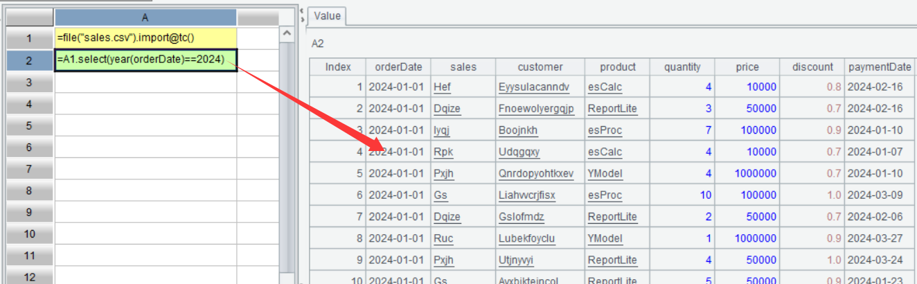
It can be seen that A2 has sales records of the year 2024. On the surface, it looks very like A1’s table sequence, but it isn’t a table sequence. It is an ordered set consisting only of records selected from A1’s table sequence. There is a special term for it in SPL – record sequence.

Get total sales, the largest single order by amount, and the number of orders in the last year

Step 1: Read data from sales.csv:

	A
1	=file(“sales.csv”).import@tc(orderDate,quantity,price,discount)

A1 As in this example only some fields (orderDate, quantity, price, discount)will be used, we specify them through parameters in import() function to retrieve only these fields during data retrieval. This way retrieval will be faster and memory usage will be lower.

Step 2: Get records of the year 2024, compute the total order amount, and add the result to the original record sequence as a computed column.

	A
1	=file(“sales.csv”).import@tc(orderDate,quantity,price,discount)
2	=A1.select(year(orderDate)==2024).derive(quantity*price*discount:amount)

A2 The derive() function adds a computed column. In the function, quantity*price*discount is a computing expression, and amount is name of the newly-generated computed column; the expression and the column name are separated by the colon. Note that the expression should be written before the column name.

Step 3: Perform aggregation.

	A
1	=file(“sales.csv”).import@tc(orderDate,quantity,price,discount)
2	=A1.select(year(orderDate)==2024).derive(quantity*price*discount:amount)
3	=A2.sum(amount)
4	=A2.max(amount)
5	=A2.count()

A3 Sum values of A2’s amount fields.

A4 Find the largest amount field value in A2.

A5 Perform count to find the number of records in A2.

Select top3 largest orders in terms of amount

	A
1	=file(“sales.csv”).import@tc()
2	=A1.select(year(orderDate)==2024).derive(quantity*price*discount:amount)
3	=A2.sort(-amount)
4	=A3.to(3)

A3 The sort() function performs sorting operation, in ascending order by default. Sorting data in descending order amounts to sorting their opposite numbers in ascending order, so a negative sign is used and the syntax is -amount.

A4 A3.to(3) selects the first records from A3. You can combine statements in A3 and A4 and write them as A2.sort(-amount).to(3).

Below is result of executing A4’s statement:

Though it is simple, this algorithm does not solve the tied rank problem. To deal with a case with probable tied ranks, SPL offers top() function:

	A
1	=file(“sales.csv”).import@tc()
2	=A1.select(year(orderDate)==2024).derive(quantity*price*discount:amount)
3	=A2.top@r(3;-amount)

A3 A2.top@r(3;-amount) sorts A2 and retrieves the first 3 records. Its default sorting rule is the same as that for the sort() function. The top() function has an @r option for handling tied ranks. It is particularly important to note that 3 and -amount are separated by the semicolon; this way it is records where amount field values ranked in top 3 that the function returns. If the separator is comma, the function only returns amount field values ranked in top 3. Unlike Excel and other programming languages, comma isn’t the only parameter separator used in SPL. There are also semicolon and colon (the previous derive() function uses the colon to separate the expression and the field name).

Below is A3’s result:

The top() function solves the tied rank problem.

Get the first/last paid order

	A
1	=file(“sales.csv”).import@tc()
2	=A1.select(year(orderDate)==2024)
3	=A2.minp(paymentDate)
4	=A2.maxp(paymentDate)

A3 A2.minp(ParmentDate) gets the record where paymentDate value is the smallest, that is, the one with the first paid order, from record sequence A2. It is basically equivalent to top(1;…). As the date value in this example is accurate to the day, there may be multiple payments in one day. To select all records where orders are paid on the same date, we can use @a option in minp() function, such as A2.minp@a(paymentDate).

A4 Select the record with the last paid order from A2. The use of maxp()function are the same as that of minp() function.

Count customers who place an order and make payment after 2025-01-01 (distinct count)

	A	B
1	=file(“sales.csv”).import@tc()	2025-05-01
2	=A1.select(orderDate>B1)
3	=A2.icount(customer)
4	=A2.select(paymentDate).icount(customer)

A3 A2.icount(customer) gets customer value from A2 row by row and then perform distinct count.

A4 A2.select(paymentDate) selects records where paymentDate isn’t null, that is, those where orders are paid.