K-means clustering results are highly sensitive to the random initialization of centroids. The results of two clustering runs may vary significantly due to differences in the initial centroids. This can lead to an undesirable situation where data from the same day is assigned to different production routes simply because of variations in the clustering process. This is unacceptable in an industrial production setting.

To avoid the impact of random centroid initialization, it’s essential to specify a definitive member as the initial centroid for k-means clustering, thus guaranteeing stable clustering results. However, how should these initial centroids be chosen?

Production routes are the categories to be clustered. The objective is to identify a representative member for each production route based on the yield data and use these representative members as the initial centroids for the k-means algorithm. But what constitutes a representative member within a specific production route?

Production routes are characterized by relatively high yields for their target outputs and comparatively low yields for the remaining outputs. Consequently, members exhibiting high yields for particular outputs and low yields for others can be deemed representative members. The problem then becomes: how to sort these production routes?

A metric is needed to measure the importance of the production routes, which is equivalent to measuring the importance of their respective outputs. In industry, priority is typically given to outputs exhibiting both high yields and high volatility. Based on this principle, we define the standard deviation of an output’s yield as a measure of its importance; specifically, the greater the standard deviation of a particular output, the more important that output is considered.

Importance ipt_j of the j-th output within yield data X:

ipt_j=std(X_j)

Based on the above approach, the centroids, C, are initialized as follows:

1. Calculate the importance of each output:

ipt_j=std(X_j)

where ipt_j is the importance of the j-th output.

Sort in descending order based on importance and record the indices Sidx:

Sidx=[a_1,a2,…,an],ipt_{a_1}>ipt_{a_2}>…>ipt_{a_n}

where a_1,a2,…,an are the indices of n outputs sorted in descending order based on importance.

2. Transpose the yield data and sort based on output importance, XT:

XT=X^T(Sidx)

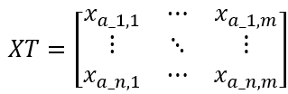
Where each row in XT represents the yield of one output, with importance decreasing from top to bottom.

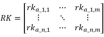
3. Calculate the rank, RK_j, for each output’s yield. A higher yield corresponds to a lower rank.

Rk_{a_j}=XT_{a_j}.ranks()

where XT_{a_j} represents the yield for the a_j-th output, and ranks() is the ranking method.

Rank matrix RK:

4. Identify candidate centroids, Cb.

Since each output potentially corresponds to a production route, we can identify representative members for all outputs to serve as the candidate centroids, Cb.

Loop through each output’s yield data. For each output, identify the data point that maximizes the difference between its rank and the sum of the ranks of all other outputs. Designate this data point as a candidate centroid, Cb_t.

Cb_t=X_h,h=pmax(rk_{a_ti}-sum([rk_{a_1i},rk_{a_2i},…,rk_{a_(t-1)i},rk_{a_(t+1)i},…,rk_ni])),i∈[1,2,…,m]\s,t∈[1,2,…,k]

Where Cb_t is the a_t-th candidate centroid (which corresponds to the t-th most important output), h is the h-th row of X (and the h-th column of RK), pmax() is the function returning the index of the maximum value, and s is the set of indices that have already been selected as centroids.

With a large number of outputs, it is possible for different clusters to have the same initial centroid. Therefore, the calculation must exclude any data points already selected as centroids; that is, i∈[1,2,…,m]\s.

Below is an explanation of why yield rank data is used in place of direct yield values.

Because the numerical values of yields for different outputs can vary significantly. For instance, diesel yield may range from 0.3 to 0.5, liquefied gas yield may only range from 0.05 to 0.1. Directly using these values in calculations can be unduly influenced by their magnitudes, hindering the accurate identification of representative members within each production route. By contrast, using yield ranks mitigates the impact of yield values, enabling more accurate identification of representative members for each production route.

If the number of clusters, k, is greater than the number of outputs, n, then loop through all data points, identifying the point that has the maximum sum of distances to the existing candidate centroids and adding it to the candidate centroid set. This process continues until k candidate centroids have been selected.

Cb_n+p=X_h,h=pmax(sum(dis(Cb_t,X_i))),p∈[1,2,…,k-n],t∈[1,2,…,n+p],i∈[1,2,…,m]

where p represents the p-th candidate centroid selected from the data points outside the initial n. This is a loop process, where the centroids identified in each loop need to be added to the existing candidate centroid set and used in subsequent loop calculations.

If the number of clusters, k, is less than the number of outputs, n, then only the k most important candidate centroids are selected as the final centroids, C.

Cb’=Cb(Sidx)

C=[Cb’₁, Cb’₂,…, Cb’_k]

where Cb’ represents the candidate centroids Cb sorted in descending order based on output importance, and C is the subset containing the top k members from Cb’.

SPL routine:

	A	B
1	[[0.113,0.345,0.316], [0.118,0.314,0.322], [0.125,0.334,0.314], [0.139,0.254,0.371], [0.111,0.361,0.306], [0.179,0.257,0.332]]	/X
2	=k=3
3	=transpose(A1)
4	=mstd@s(A3,2)
5	=A4.psort@z()	/Sidx
6	=A3(A5).(~.ranks())	/RK
7	=as=to(A6.len()),av_idx=to(A1.len()), A6.((oidx=as\#,pma=(~--msum(A6(oidx),1).~)(av_idx).pmax(), res=av_idx(pma),av_idx.delete(pma),res))	/Cb index
8	=A1(A7)	/Cb’
9	for k-A5.len()	=A1.pmax((v=~,A8.sum(dis(~,v))))
10		=A1(B9)
11		=A8.insert(0,[B10])
12	=if(k<A7.len(),A8.to(k),A8)	/Initialized centroids C
13	=k_means(A1,k,300,A12)

Calculation result example:

Yield data X:

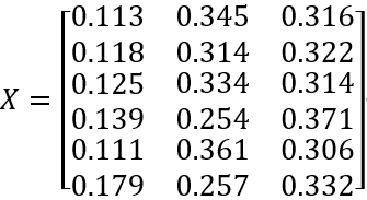
As the yield data encompasses only the yields of the primary outputs, the cumulative yield is not equal to 1. Consequently, practical applications focus solely on clustering these primary outputs.

Number of clusters k=3

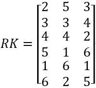
Rank matrix RK:

Output importance IPT:

IPT=[0.0257, 0.0455, 0.0233]

Sidx: Indices resulting from sorting IPT in descending order:

Sidx=[2,1,3]

Initialized centroids C:

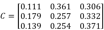
We can see that, for C₁, the yield of the 2nd output is maximal among the three centroids; for C₂, the yield of the 1st output is maximal; and for C₃, the yield of the 3rd output is maximal. Furthermore, the indices of these maximal values, [2,1,3], exactly correspond to Sidx.

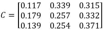
Centroids obtained after k-means clustering:

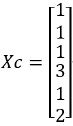
Cluster assignments for members in X, Xc: