

7.1 Output yield and production route
In industrial settings, the output yields of certain units often exhibit significant fluctuations, and some of these outputs require special attention. These outputs of interest are often associated with specific production routes. For example, in a catalytic cracking unit, a high gasoline yield indicates a gasoline route, while a high diesel yield indicates a diesel route. The goal is to classify historical yield data into a specified number of clusters, so that these clusters correspond to the respective production routes. Subsequently, when modeling (e.g., building a linear model under mass conservation constraints), data from the same production route are selected as input data to improve model accuracy.
The yield data of different outputs for a given input is represented by X:
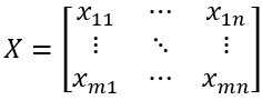
where n is the number of outputs and m is an index. Each row represents the yields of different outputs for a particular day’s production data, and each column represents the daily yields of a specific output.
Our aim is to classify the yield data, X. However, since the historical data lacks pre-existing labels, unsupervised clustering is necessary. Given that the number of production routes corresponds to the number of clusters, k-means clustering satisfies our requirements.
Classifying the yield data, X, into k clusters is performed as follows:
1. Randomly select k data points as initial cluster centroids C:
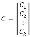
where Ct is the centroid of the t-th cluster in C, chosen randomly from X.
2. Calculate the distance from each data point to the k centroids. Assign each data point to the k-th cluster whose centroid is closest:
xci=t,t=pmin(dis(Xi,Ct))
where xci is the cluster label for the i-th row Xi of X, Ct is the centroid of the t-th cluster, and dis() is the distance calculation method.
Yields from the same production route are similar. If each row in X is viewed as a point in a high-dimensional space, points from the same production route should cluster together, while points from different production routes should be relatively far apart. Therefore, we choose Euclidean distance as the distance metric.
3. Update the centroids.
Compute the mean yield of each output yield in each cluster and use them as the new centroids, CN:
CNt=avg(Xtj),j∈[1,2,…,n],t∈[1,2,…,k]
where CNt is the new centroid of the t-th cluster, and Xtj is the yield of the j-th output from data points in X that belong to the t-th cluster.
4. Repeat steps 2 and 3 until the centroids no longer move or the maximum number of iterations N is reached.
That is, the sum of the distances between the centroids is less than a very small threshold, ε:
sum(dis(CNt, COt))<ε|| iter==N,t∈[1,2,…,k]
where COt is the centroid of the t-th cluster from the previous iteration, ε is a very small number, iter is the number of iterations, and dis() is the distance calculation method.
Upon completion of the iterations, each point in X is assigned to the cluster associated with the nearest centroid, Ct.
xci=t,t=pmin(dis(Xi,Ct))
SPL routine:
| A | B | C | D | |
|---|---|---|---|---|
| 1 | [[1,2,3,4],[2,3,1,2],[1,1,1,-1],[1,0,-2,-6]] | /X | ||
| 2 | =k=2 | /Number of clusters | ||
| 3 | =iter=300 | /Number of iterations | ||
| 4 | =center=null | /Initial centroids C | ||
| 5 | =it=0 | |||
| 6 | =func(A7,A1,A2,A3,A4) | |||
| 7 | func | |||
| 8 | if !D7 | =D7=A7.sort(rand()).to(k) | /Random centroids | |
| 9 | =it+=1 | |||
| 10 | return func(A7,A7,B7,C7,D7) | |||
| 11 | else | =A7.((d=~,D7.(dis(~,d)))) | ||
| 12 | =C11.(~.pmin()) | |||
| 13 | =A7.group(C12(#)) | |||
| 14 | =C13.((cent=mmean(~,1).~,if(ifa(cent),cent,[cent]))) | |||
| 15 | =C14.sum(dis(~,D7(#))) | /Sum of distances between new and old centroids | ||
| 16 | 1E-4 | /ε | ||
| 17 | if C15<C16||it==C7 | |||
| 18 | =C14 | |||
| 19 | =C12 | |||
| 20 | return [D18,D19] | |||
| 21 | else | =D7=C14 | ||
| 22 | =it+=1 | |||
| 23 | return func(A7,A7,B7,C7,D7) | |||
Calculation result example:
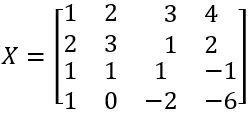
Input data X:
Number of clusters, k=2
Maximum number of iterations, iter=300
Clustering results:
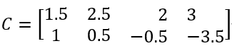
Centroids C:
Cluster assignments, Xc:
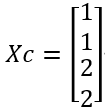
It is easy to verify that X1 and X2 are closer to C1, therefore their mean is C1. Similarly, X3 and X4 are closer to C2, and their mean is C2.
SPL Official Website 👉 https://www.esproc.com
SPL Feedback and Help 👉 https://www.reddit.com/r/esProcSPL
SPL Learning Material 👉 https://c.esproc.com
SPL Source Code and Package 👉 https://github.com/SPLWare/esProc
Discord 👉 https://discord.gg/sxd59A8F2W
Youtube 👉 https://www.youtube.com/@esProc_SPL

