The bounded linear fitting method ensures that yields remain within defined boundaries during fitting, and the error limitation method prevents excessive deviation from the baseline yield. However, Constraint 2—that the sum of yields for all outputs from a given input must equal 1—is still not satisfied. This section presents a linear transformation method to satisfy this constraint, thereby obtaining the final yield, W.

The baseline output matrix, denoted YB, is obtained using the input matrix X and the baseline yields B:

YB=X*B

The deviation matrix, E, is obtained by comparing Y and YB:

E=Y-YB

The deviation yield boundary BD is calculated using the error limitation method:

BD=bd(X,Y,B,rg)

where bd(…) represents the error limitation method, and rg is the boundary adjustment ratio, rg∈[0,1].

The bounded linear fitting algorithm is used to fit X and E, obtaining the deviation yields, denoted WE:

WE=BDfit(X,E,BD)

where BDfit(…) is the bounded linear fitting algorithm.

WE does not guarantee that W satisfies Constraint 2. However, a linear transformation can be applied to obtain the best deviation yield, WD, that satisfies the constraint while minimizing the loss of accuracy.

WD=L(WE)

where L(…) represents a certain linear transformation.

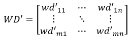
We expect that summing WD and the baseline yield B will obtain the yield W. Consequently, the constraints on W are transformed into constraints on WD, as shown in the figure below.

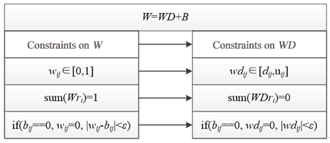
d_ij and u_ij are the upper and lower bounds, respectively.

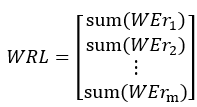
Ideally, the row sum WRL of WE is 0, which means that each column of WE has a linear relationship with the sum of the other columns.

This linear relationship can be used to perform a linear transformation on WE to obtain WD that satisfies Constraint 2.

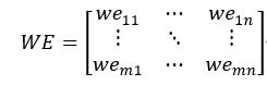
Assume the WE matrix is as follows:

(1) Calculate the row sums, WRL, of WE:

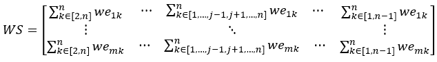
(2) Calculate the matrix WS, formed by the sums of the vectors in WE excluding the j-th column:

(3) Obtain WD through linear transformation:

WEc_j, WSc_j and WRL have the following relationship:

WEc_j+WSc_j=WRL

Given that WEc_j represents the optimal yield for the j-th column as determined by the bounded linear fitting algorithm, it follows that WSc_j=WRL-WEc_j is also accurate. Apply the following linear transformation to obtain WD’:

WD’c_j=WEc_j*(n-1)/n+WSc_j*(-1/n)

=WEc_j*(n-1)/n+(WEc_j-WRL)/n

=WEc_j-WRL/n

where WD’c_j denotes the element in the j-th column of the linearly transformed matrix WD’.

After linear transformation, it is equivalent to subtracting the row mean WRL_i from a certain deviation yield we_ij:

wd’_ij=we_ij-WRL_i/n

WD’ satisfies Constraint 2, but it is still necessary to verify whether WD’ allows W to satisfy Constraint 1, i.e., whether w_ij=wd’_ij+b_ij ∈[0,1].

If W satisfies constraint 1, then the fitting is complete:

WD=WD’

If there exists a wd’_ij such that w_ij ∉[0,1], then the transformation rule needs to be adjusted.

Assume that there are z columns in WE that have elements that do not satisfy the constraint:

WE=[WEc₁,WEc₂,…,WEc₍₁₎,…,WEc_(z),…,WEc_n]

where [WEc₍₁₎,…,WEc_(z)] are the columns of deviation yield that, even after transformation, still do not meet the constraint. That is, there exists:

we_i(p)+b_i~(p)~∉[0,1]，p∈[1,z]

The previous linear transformation was WD’c_j=WEc_j*(n-1)/n+WSc_j*(-1/n). The transformation coefficients for both were fixed at (n-1)/n and (-1/n), but because the constraint cannot be satisfied, this cannot be used. Another approach is to fix the transformation coefficient of WEc_j to 1 and solve for the coefficient of WSc_j using an equation.

Let the coefficient vector for WSc_j be vector A, as given by the equations below:

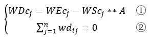
where WDc_j is the j-th column element of the deviation coefficient matrix WD.

The coefficient vector A can be obtained from equations ① and ②. Additionally, the yield we_ij must also equal 0 when the baseline yield b_ij equals 0.

Solving the equations obtains the vector A:

After obtaining vector A, substitute it into Equation ① to get WDc_j.

At this point, it is necessary to re-verify whether WD allows W to satisfy Constraint 1. If it does, the calculation is complete, and WD is obtained. Otherwise, the columns that do not satisfy the constraint condition must be added to the set [WEc₍₁₎,…,WEc_(z)], and the above method is repeated until all w_ij satisfy Constraint 1 (w_ij=(wd_ij+b_ij)∈[0,1]), yielding WD.

Finally, add the base yield matrix B to WD to obtain W:

W=B+WD

SPL routine:

	A	B	C	D
1	[[30,8],[31,7],[38,10]]		/X
2	[[2,13,23],[3,15,20],[11,13,24]]		/Y
3	[[0,0.5,0.5],[0.55,0.05,0.4]]		/B
4	0.1		/rg
5	=mul(A1,A3)		/X*B
6	=A2.(~–A5(#))		/E
7	=bd(A1,A2,A3,A4).(.(.(round(~,3))))		/BD
8	=A6.~.((idx=#,bdfit(A1,A6.([~(idx)]),A7.(~(idx))).conj()))			/WET
9	=transpose(A8)		/WE
10	=func(A12,A9,A3)		/WD
11	/Linear transformation; parameters: WE, B
12	func
13		=A12.(~.count(~==0))		/Number of zeros in each row of WE
14		=A12.~.len()		/Number of outputs
15		=A12.((s=~.sum(),ind=#,~.(if(~==0,0,s/(B14-B13(ind))))))		/Calculate mean per row
16		=A12.(~–B15(#))	/weij-WRLi/n
17		=B12.(~++B16(#))	/W=WD’+B
18		=transpose(B17)
19		=B18.pselect@a(~.pselect(~<0||~>1)>0)	/Record column indices where WD’ violates constraints
20		if B19.len()==0	return B17	/If no violations, return W
21		else	=func(A24,A12,B12,B19)	/If violations, adjust transformation rule
22			return C21
23	/Recursive elimination of elements violating Constraint 2
24	func
25		=B24.~.len()
26		=A24.(~.sum())		/WRL
27		=A24.((w=~,w.((ind=#,if(~==0,0,w(to(B25).delete(ind)).sum())))))		/WS
28		=A24.(~.pselect@a(~==0))	/Indices where the yield is 0 in WEri
29		=B28.(~&C24)	/Indices that are zero and violate constraints
30		=B26.(~/((B25-B29(#).len()-1)*~+A24(#)(B29(#)).sum()))		/ai
31		=A24.((ind=#,~.(if(B29(ind).pos(#)>0,0,B30(ind)))))		/A
32		=B27.(~**B31(#))		/A**WScj
33		=A24.((idx=#,if(B31(#).id()==[0],B32(#),~–B32(#))))		/WD
34		=B24.(~++B33(#))		/B+WD
35		=transpose(B34)		/WT
36		=B35.pselect@a(~.pselect(~<0||~>1)>0)	/Re-check for any yields violating constraints
37		if B36.len()==0	return B34	/If no violations, return W
38		else	=C24=C24&B36	/If violations, record them
39		=func(A24,A24,B12,C24)		/WD

bd(…) in cell A7 is the error limitation method used to calculate the deviation yield boundary BD.

bdfit(…) in cell A8 is the bounded linear fitting algorithm.

The code block in cell A12 performs a linear transformation on WE.

The code block in cell A24 performs a transformation on WD’.

Calculation result example:

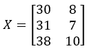
Input X:

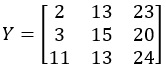
Output Y:

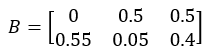
Baseline yield B:

Boundary adjustment ratio rg:

rg=0.1

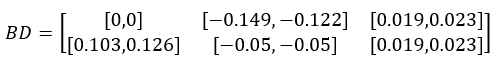
Calculated boundary BD:

Final yield W:

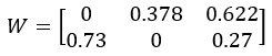
Let’s start by looking at the MSE for each output using the baseline yield B:

MSE₁=12.24

MSE₂=16.24

MSE₃=8.98

where MSE_j is the MSE for the j-th output.

Now, let’s examine the MSE for each output using W:

MSE₁=10.97

MSE₂=5.13

MSE₃=3.86

It is evident that the fitted W yields a better result.