Having accumulated some sample data for inputs and outputs, we want to calculate the yield matrix.

If there are no constraints, we can obtain the yield W using the least squares method:

W=linefit(X,Y)

Where linefit(…) is the least squares linear fitting function.

At this point, W is unconstrained, and its elements may be greater than 1 or less than 0. This is meaningless for production, so when considering Constraint 1, simply using least squares is not feasible.

If only Constraint 1 (0 and 1 are the boundaries for w_ij) is considered, the goal is to minimize the mean squared error (MSE) within those bounds:

MSE=(Y-XW)²

w_ij ∈[0,1]

It can be proved that the optimal solution is either on the boundary or at the least-squares fit value. Thus, w_ij has three possible values:

w_ij=0

w_ij=1

w_ij=linefit(…), and w_ij ∈[0,1]

When the number of inputs is limited, we can find the optimal solution by exhaustively enumerating the three possible yield values for each input. This leads to 3^m combinations for m inputs. The yield set that minimizes MSE within the boundary is the optimal solution. We call this the Bounded Linear Fitting algorithm.

We will now describe the Bounded Linear Fitting algorithm, using the first output column, Yc₁, as an example. The process is the same for all other inputs.

1. Exhaustively enumerate all possible values for the input yields

Each input yield has three possible values. With m inputs, this is equivalent to m nested loops, resulting in 3^m possible yield combinations, which we denote as s.

s=3^m

For example, when all input yields take the least-squares fitted value:

W(t) =linefit(X,Yc₁)

Where W(t) is the t-th yield matrix for Yc₁, with t∈[1,s].

When all input yields take the lower bound:

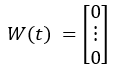
In this case, the yield matrix is an m*1 matrix consisting of m zeros. Similar situations arise when other yield values reach the boundary; the boundary value then reflects the yield for that input.

When only some input yields take boundary values:

The yields for the remaining inputs are determined using the least-squares method. If the yields of inputs Xc_a,Xc_b,…,Xc_l are at their boundary values, then those yields are Wr_a,Wr_b,…,Wr_l, respectively.

Let X’ represent the inputs whose yields are not at their boundary values. The corresponding outputs, denoted as Yc₁’, are then calculated by subtracting the product of the boundary yields and their respective inputs.

Yc₁’=Yc₁-(Xc_a*Wr_a+Xc_b*Wr_b+…+Xc_l*Wr_l)

The yield matrix for X’, obtained via least-squares fitting, is denoted as W(t)’:

W(t)’=linefit(X’,Yc₁’)

W(t)’ and W_aj,W_bj,…,W_kj together constitute the t-th yield matrix W(t).

After exhaustively enumerating all possibilities, we obtain s yield matrices. From these, we find the yield matrix that satisfies the boundary constraints (i.e., w_ij ∈[0,1]) and has minimum MSE. This is the optimal yield.

2. Select the set of yield matrices, denoted [W]’, that meet the specified boundary conditions

Denote the set of s yield matrices as [W]:

[W]=[W(1),W(2),…,W(s)]

[W]’=[W].select(0≤W(t)_i ≤1)

Where W(t)_i represents the yield of the i-th input within the matrix W(t).

3. Calculate the MSE between each set of yield matrix in [W]’ and Yc₁.

MSE=(Yc₁-XW*(t))²

The W(t) with the minimum MSE is the optimal yield matrix Wr₁.

SPL routine:

	A	B	C	D
1	[[1,2],[1,3],[1,4]]	/X
2	[[0.3],[2.4],[1.6]]	/Y
3	[[0,1],[0,1]]	/BD
4	[0,1,2]	/0: Least squares fitted value, 1: Lower bound, 2: Upper bound
5	=(A1.~.len()-1).iterate(A4.conj((idx=#,~~.([A4(idx)].insert(0,~)))),A4)		/3m possible value makers
6	=A5.(func(A12,A1,A2,A3,~))		/[W]
7	=A6.select((w=~.conj(),w.id(between(~,A3(#)(1):A3(#)(2)))==[true]))		/[W]’ satisfying boundary constraints
8	=A7.(mse(mul(A1,~),A2))		/MSE
9	=A8.pmin()	/Index of W(t) with minimum MSE
10	=A7(A9)	/Optimal W
11	/Calculate W(t); Parameters: X, Y, Boundaries, 1 value maker
12	func
13		=D12.align@ap([true,false],~!=0)
14		=B13(1)	/Input number taking boundary value
15		=D12(B14)	/Upper bound, lower bound, or least squares fitted value?
16		=B13(2)	/Input number not taking boundary value
17		=C12(B14)
18		=B17.([~(B15(#))])	/[Wra,Wrb,…,Wrl]
19		if B16.len()==0	return B18	/All inputs take boundary values
20		=A12.(~(B14))	/[Xca,Xcb,…,Xcl] taking boundary values
21		=if(B18.len()<1,B12.([null]),mul(B20,B18))	/Xca*Wra+Xcb*Wrb+…+Xcl*Wrl
22		=B12.(~–B21(#))	/Ycj’
23		=A12.(~(B16))	/X’ not taking boundary values
24		=w=linefit(B23,B22),if(ifnumber(w),[[w]],w)	/W(t)’
25		=B18|B24	/Combine [Wra,Wrb,…,Wrl] with fitted W(t)’
26		=B13.conj()	/Input index
27		=B26.psort()	/Original input order
28		=B25(B27)	/Processed W(t)
29		return B28

This routine explains the single-output scenario. The multi-output scenario is similar, simply involving more loops.

A5 utilizes the iterative function iterate(…) function to create 3^m possible value markers.

The markers in A4 represent three possible scenarios: 0 signifies the need for least squares fitting, 1 the lower bound, and 2 the upper bound. With two columns of inputs in this example, there are 9 possible marker combinations, as detailed in the following table:

No.	Marker combination	Column 1 input	Column 2 input
1	[0,0]	Least squares fitting	Least squares fitting
2	[0,1]	Least squares fitting	Lower bound
3	[0,2]	Least squares fitting	Upper bound
4	[1,0]	Lower bound	Least squares fitting
5	[1,1]	Lower bound	Lower bound
6	[1,2]	Lower bound	Upper bound
7	[2,0]	Upper bound	Least squares fitting
8	[2,1]	Upper bound	Lower bound
9	[2,2]	Upper bound	Upper bound

The code block in A12 calculates the optimal yield matrix W for output Y.

Calculation result example:

Let’s start by looking at the results of applying least squares fitting to the above X and Y:

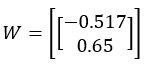
The MSE for this yield, W, is:

MSE=0.467

Now, let’s examine the fitting results of the bounded linear fitting algorithm:

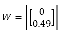
The MSE for this yield, W, is:

MSE=0.486

While least squares fitting produces a better MSE, its failure to meet boundary constraints renders it impractical for actual production. Therefore, the bounded linear fitting algorithm is the preferred choice.