For time series, comparing the similarity of two time series is a common task. Intuitively, the closer the data points of two time series are, the more alike their graphs appear, and thus the greater the similarity between the time series. The degree to which they resemble each other is quantified as a similarity score, denoted as sm.

Assuming the similarity between two time series, A and B, can be calculated using a mathematical method, represented as Sim(…), then:

sm=Sim(A,B)

Theoretically, Sim(…) can take infinitely many forms. We will now introduce a simple and effective method: Dynamic Time Warping (DTW).

If two time series are perfectly aligned (with close values at corresponding points), we can simply calculate the sum of distances (e.g., absolute differences) between corresponding points, as illustrated in the figure below with two time series:

Time series A and B in figures (a) and (b) are perfectly aligned and highly similar. Their similarity, denoted as sm, can be calculated simply by summing the distances between corresponding points.

sm=sum(|A_i-B_i|),i∈[1,n]

Where A_i is the i-th element of A, B_i is the i-th element of B, and n is the number of elements in A and B.

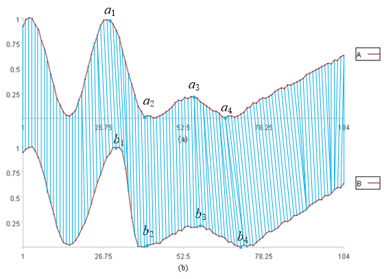
In practice, time series are rarely perfectly aligned, yet they may still appear visually similar. Consider, for example, the two time series in figures (a) and (b) below:

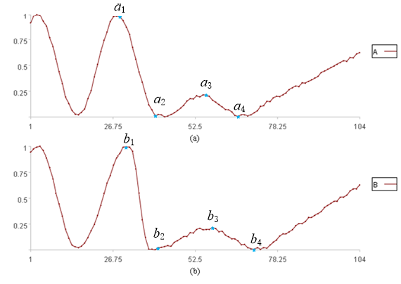
In figures (a) and (b), the two time series share a generally similar shape, but are not perfectly aligned on the x-axis. Ideally, a1, a2, a3, a4 from A would correspond to b1, b2, b3, b4 from B; however, this is clearly not the case in the figure. Consequently, directly calculating the sum of distances between corresponding data points may not accurately reflect their similarity. How should we proceed in such cases?

Prior to comparing the similarity of two time series, one (or both) of the time series must be warped along the x-axis to achieve alignment.

So, how can two time series be aligned? In other words, what constitutes a correct warping? Intuitively, a correct warping allows one series to coincide with the other, thereby minimizing the sum of distances between all corresponding points of the two time series.

Suppose we have two time series, A and B, each of length n (although DTW can handle unequal lengths with the same algorithmic process; for simplicity, we will focus on equal-length series, which are more common in practice).

A= [a₁,a₂,…, a_n]

B= [b₁,b₂,…, b_n]

We continue to use the distance between points in the two time series as a measure of similarity. However, because the x-axis can be warped, we do not necessarily calculate distances between sequentially corresponding points. Rather, a single point in one series may correspond to multiple points in the other, as illustrated in the figure below.

Of course, constraints apply to the warping of the x-axis:

1. Every point must be included; no point may be omitted.

2. The order of the data points in the time series must remain unchanged.

3. Although a ‘one-to-many’ relationship is allowed, crossing is prohibited.

If the length of the time series is finite, the number of possible x-axis warps is theoretically finite. Although we could exhaustively evaluate each warping and select the one yielding the minimum distance, this is computationally extensive. Therefore, we employ dynamic programming for efficient calculation.

To align the two series, we need to construct an n*n distance matrix D, where element d_ij represents the distance between points a_i and b_j. (i.e., the distances between every point in time series A and every point in time series B; smaller distances indicate higher similarity, disregarding order for now). Typically, the absolute difference, d_ij= |a_i-b_j|, is used to define the distance between two points. Each element in the matrix represents an alignment between points a_i and b_j. The DTW algorithm aims to find an optimal path through the distance matrix, such that the points on the path define the aligned points used for similarity calculation, as illustrated below.

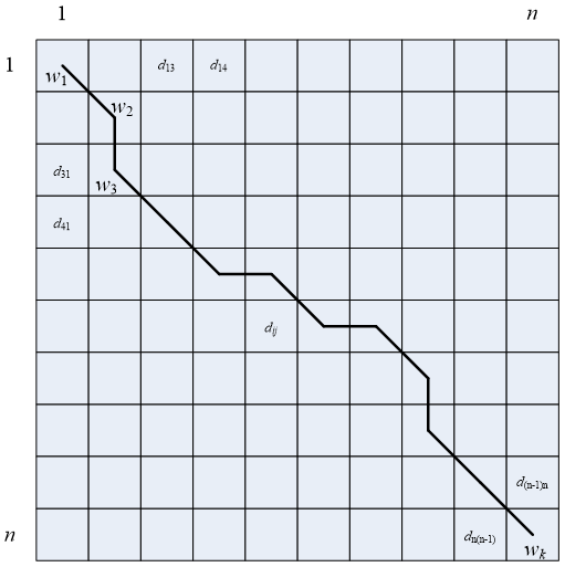
Assuming the grid above represents the distance matrix D, with each cell being a matrix element d_ij, and the solid line W representing the path of shortest cumulative distance, how can we find this path W?

We designate this path as the warping path, denoted by W. The k-th element of W is defined as w_k= (i,j), which specifies the correspondence between elements a_i and b_j. That is:

W=[w₁,w₂,…,w_k],k∈[n,2*n-1]

This path is not selected arbitrarily, but rather is subject to the following constraints:

1. Boundary condition

These two time series A and B must have corresponding start and end points. Specifically, a₁ must correspond to b₁, and a_n to b_n. Therefore, any chosen path must begin in the upper left corner and end in the lower right corner; that is, w₁=(1,1),w_n=(n,n).

2. Continuity

Given that w_m-1=(a’,b’), the subsequent point on the path, w_m=(a,b), must satisfy (a-a’)≤1 and (b-b’)≤1. This means alignment cannot skip points; it must occur with adjacent points only. This guarantees that every coordinate of A and B appears in W.

3. Monotonicity

If w_m-1=(a’,b’), then the subsequent point on the path, w_m=(a,b), must satisfy (a-a’)≥0 and (b-b’)≥0. This ensures that the points along path W increase monotonically with time.

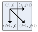
Subject to the continuity and monotonicity constraints, there are only three possible directions from each grid point along the path. For instance, if the path currently passes through grid point (i, j), the next grid point on the path must be one of (i+1, j), (i, j+1) or (i+1, j+1), as illustrated in the figure:

Given the aforementioned constraints, there exist approximately 3ⁿ possible warping paths. We aim to minimize the accumulated distance along the path W. This minimum distance is then used as a measure of similarity, sm, between time series A and B.

sm=min(sum(D(w_i)))/n

Where D(w_i) represents the distance value taken from the distance matrix D at the location specified by w_i, and division by n yields the average distance.

To find the path W with the minimal accumulated distance, we define a cumulative distance matrix C. Beginning at point (1, 1), representing the initial alignment between A and B, we iteratively sum the distances along the path. The final value at the end point (n, n) represents the total accumulated distance, which we use as the similarity score, sm, between A and B.

The cumulative distance c_ij is defined as the sum of the current distance d_ij (the element at row i, column j of the distance matrix D) and the minimum cumulative distance from any reachable neighbor.

c_ij=α*d_ij+min(c_(i-1)(j-1), c _(i-1)j,c _i(j-1))

Where α is a penalty coefficient used to penalize different paths. To discourage one-to-many correspondences between the two time series, a higher α value (e.g., α>1) is applied to segments of paths exhibiting such correspondences.

The optimal warping path W is the path that minimizes the cumulative distance, and this minimum distance defines the similarity between time series A and B.

sm=c_kk/n

SPL routine:

	A	B	C	D	E
1	[2,1,5,2,4]	/A
2	[1,5,5,3,5]	/B
3	1	/Penalty coefficient α
4	=A1.((v=~,A2.(abs(~-v))))			/Distance matrix D
5	=A4.(~.(null))			/Initialize the cumulative distance matrix C
6	=CD=[]	/Record path
7	for A4.len()	for A4(1).len()	/Loop through each element in D
8			=A7-1	/i-1
9			=B7-1	/j-1
10			=[C8,C9]	/(i-1,j-1)
11			=[C8,B7]	/(i-1,j)
12			=[A7,C9]	/(i,j-1)
13			=[C10,C11,C12]	/Possible three cases
14			if C8==0&&C9==0	=D26=0	/When processing the first element
15				=D25=C10
16			else if C8==0	=D26=A5(A7)(C9)	/When processing elements in the first row
17				=D25=C12
18			else if C9==0	=D26=A5(C8)(B7)	/When processing elements in the first column
19				=D25=C11
20			else	=A5(C8)(C9)	/When processing other elements
21				=A5(C8)(B7)
22				=A5(A7)(C9)
23				=[D20,D21,D22]	/Possible paths
24				=D23.pmin()
25				=C13(D24)
26				=D23(D24)
27			=if(D25==C10,1,A3)	/Penalty coefficient α
28			=CD.insert(0,[D25])	/Record path
29			=A4(A7)(B7)	/Distance dij
30			=D26+C29*C27	/Cumulative distance cij
31			=A5(A7)(B7)=C30	/Update the cumulative distance matrix C
32	=A6.group((#-1)(A4.~.len()))			/Path matrix
33	=path=[[A4.len(),A4.~.len()]]			/Initialize the path sequence
34	=A6.m(-1)
35	for	=path.insert(0,[A34])		/Record path in reverse
36		=A34(1)
37		=A34(2)
38		if B36==1&&B37==1	break
39		=A32(B36)(B37)
40		=A34=B39
41	=path.rvs()	/Path
42	=A5.m(-1).m(-1)/A1.len()			/Distance (similarity)

Calculation result example:

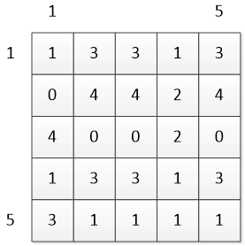
Distance matrix D:

Cumulative distance matrix C:

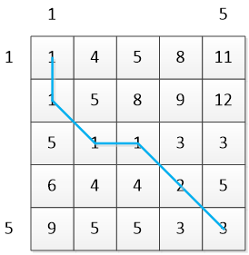
The blue line in the figure is the optimal path W:

W=[(1,1),(2,1),(3,2),(3,3),(4,4),(5,5)]

The final curve similarity, sm:

sm=3/5=0.6

Correspondence between two time series:

Aligned time series:

Time series A and B are displayed in Figure (a), while their aligned counterparts, A2 and B2, are presented in Figure (b). As the figures demonstrate, the two time series exhibit a strong degree of similarity even after alignment.

The example routine calculates the similarity of time series A and B using their original values. In practice, however, the two time series may have different units of measure, so standardization (methods described in Section 4.2 of Chapter 4) is often required before using DTW to compute their similarity.

The DTW algorithm can also be used to calculate the similarity of curves in multi-dimensional space. The only change is that the distance metric needs to be redefined (e.g., using Euclidean distance); the rest of the calculation process remains the same.