Points in a multidimensional space may be either clustered or scattered. How do we measure the ‘degree of dispersion’ of points distributed in space?

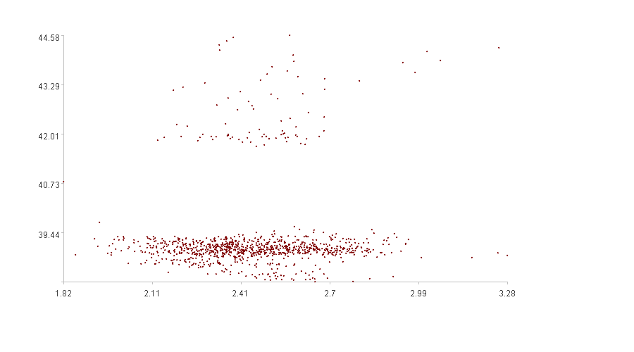
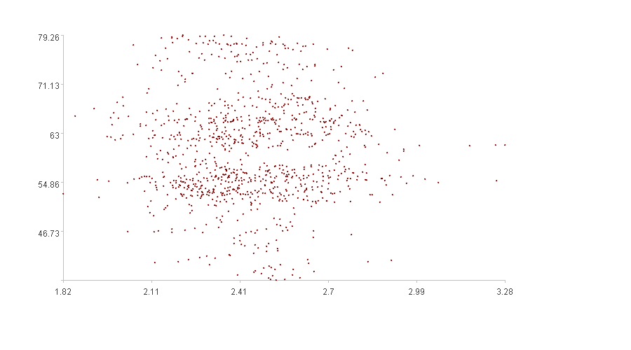
Let’s look at the two figures. The first exhibits an obvious clustering effect, with most points clustered at the bottom and a few scattered at the top, indicating a low “degree of dispersion”; the second shows less obvious clustering effect, with points scattered throughout the space, indicating a high “degree of dispersion”.

The metric describing the ‘degree of dispersion’ of points distributed in a multidimensional space is called spatial dispersion. The higher the spatial dispersion, the more dispersed the distribution, and the worse the clustering effect. Conversely, the more concentrated the distribution, the more obvious the clustering effect.

Spatial dispersion can be described as follows: Divide a multidimensional space into several small sub-spaces. When points are evenly distributed across these sub-spaces, the spatial dispersion is high. When points are concentrated in only a few sub-spaces, the spatial dispersion is low.

Information entropy is a metric describing the uncertainty of the occurrence of each possible event of an information source. The higher the uncertainty, the greater the information entropy; the lower the uncertainty, the smaller the information entropy. Spatial dispersion is a metric describing the variation in probability of a point falling into sub-spaces. The smaller the variation in these probabilities (the higher the uncertainty), the higher the spatial dispersion; the greater the variation in these probabilities (the lower the uncertainty), the lower the spatial dispersion. Therefore, we can use the information entropy formula to calculate spatial dispersion.

H(U)=sum(-P(u)*log₂(P(u))),u∈U

Where H(U) is the information entropy, U is the set of all events, u is a particular event, and P(u) is the probability of event u occurring.

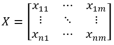
Multidimensional time series X

1. Even division of each dimension

Divide each dimension evenly into h segments, the entire space will be divided into h^m sub-spaces.

P^(j)=[p^(j)₁,p^(j)₂,…,p^(j)_h]

p^(j)_l=min(Xc_j)+(max(Xc_j)-min(Xc_j))/h*(l-1)，l∈[1,h]

Where P^(j) is the sequence of division points for the j-th dimension time series, and p^(j)_l is the value of the l-th division point when Xc_j is evenly divided.

2. Label points with location information according to the divided space

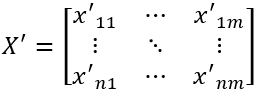
x_ij’=P^(j).pseg(x_ij)

Where x_ij’ is the position of x_ij in P^(j). For example, if p^(j)₁≤x_ij< p^(j)₂, then x_ij’=1, indicating that x_ij is in the first segment of the j-th dimension.

3. Count the number of points in each sub-space

Sp=X’.group(~)

spd_s=count(sp_s)

Where Sp is the set of sub-spaces containing points, with each set representing one sub-space, and spd_s is the number of points in the s-th set (sps). We know that the total number of sub-spaces is h^m, but some sub-spaces may not contain any points. Therefore, in general, the number of sets in Sp is less than h^m.

4. Probability of a point falling into each sub-space

Take the ratio of the number of points falling into each sub-space to the total number of points as the probability of falling into that sub-space.

spp_s=spd_s/n

Where spp_s is the ratio of the number of points falling into the s-th set to the total number of points.

5. Information entropy

etp=sum(-spp_s *log₂(spp_s))

6. Spatial dispersion

Information entropy has a characteristic: the more sub-spaces containing points, the higher the information entropy. In general, the more sub-spaces each dimension is divided into, the more sub-spaces containing points. When the number of segments per dimension is the same, more dimensions result in more sub-spaces, leading to higher information entropy. To eliminate the influence of the number of dimensions on information entropy, we can divide by a dimension-related value, which is defined as the spatial dispersion.

dsp=etp/-log₂(1/n)

SPL routine:

	A	B
1	=file(“DSP0.csv”).import@tci()	/First dimension data
2	=file(“DSP1.csv”).import@tci()	/Second dimension data
3	10	/Number of segments per dimension
4	=[A1,A2]	/XT
5	=A4.(~.max())
6	=A4.(~.min())
7	=A6.((idx=#,m=(A5(#)-~)/A3,mi=~,A3.(mi+m*(#-1))))	/P(j)
8	=A4.((idx=#,~.(A7(idx).pseg(~))))	/X’T
9	=transpose(A8)	/X’
10	=A9.group(~)
11	=A10.(~.len()/A9.len())	/Probability spps
12	=-A11.sum(if(~==0,0,~*lg(~,2)))	/Information entropy
13	=n=power(A3,A4.len()),A12/(-lg(1/n,2))	/Spatial dispersion

Calculation result example:

The first figure is a two-dimensional graph representing data from ‘DSP0.csv’ and ‘DSP1.csv’. The calculated spatial dispersion is 0.560.

The second figure is a two-dimensional graph representing data from ‘DSP0.csv’ and ‘DSP2.csv’. The calculated spatial dispersion is 0.818.

The calculation results match our intuition that the spatial dispersion of the second figure is greater than that of the first figure.