Single-dimensional anomaly detection algorithms can get alarm intensities for individual time series. By ‘aggregating’ the alarm intensities of multiple dimensions using some method, we can obtain an alarm intensity for multidimensional time series. We will introduce a simple and straightforward method to accomplish this ‘aggregation’: calculating a weighted average of the alarm intensities of all dimensions.

AW_i=sum(Wr_i **Hr_i)

Where AW_i is the aggregated alarm intensity at the i-th time point, W_ri is the alarm intensity at the i-th time point obtained from applying a single-dimensional algorithm to the m-dimensional time series, and H_ri is the weight corresponding to the m-dimensional time series at the i-th time point.

Where do these weights come from?

(1) Process knowledge

Extensive process knowledge exists in industrial production. This knowledge often includes information on the relative importance of correlated time series. Consulting relevant documentation or process experts can obtain relatively accurate weights.

(2) Algorithmic calculation

Of course, process knowledge is often incomplete; deriving weights from historical data is generally more reliable. Before outlining specific weight calculation methods, let’s look at a story.

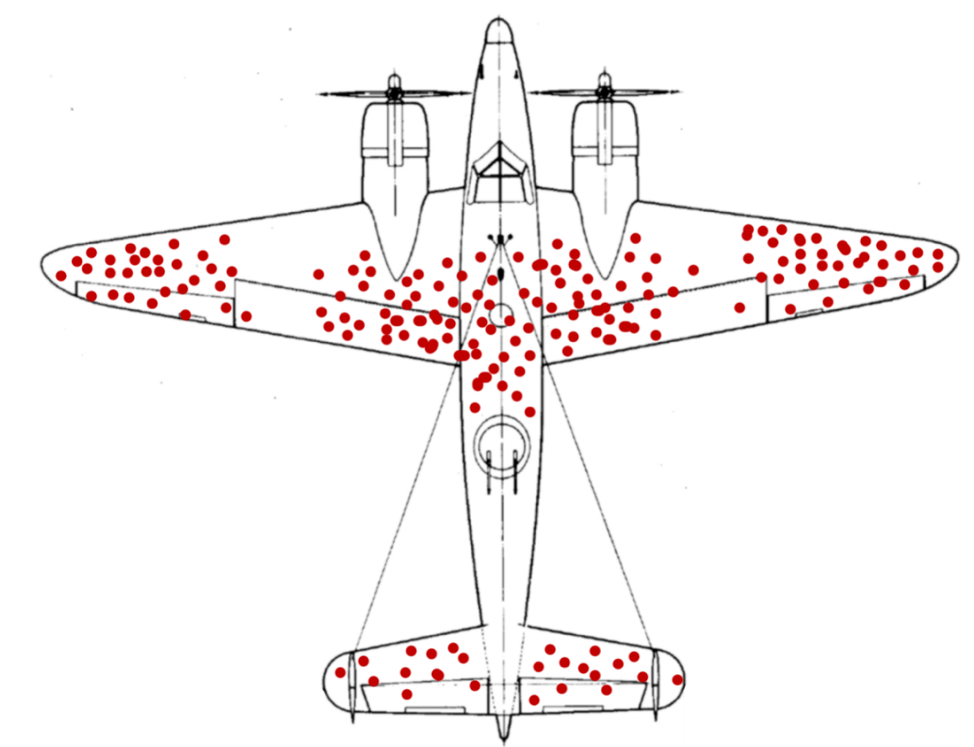
The figure above shows the distribution of bullet holes on an Allied aircraft returning from missions during World War II. As can be seen from the figure, the distribution is uneven: wings had more bullet holes, while engines had fewer. At the time, the prevailing view among military officials was to reduce overall armor and reinforce the most frequently hit areas, thereby lightening the aircraft while maintaining protection through increased efficiency. However, they were unsure how much armor to add to these areas, so they consulted Abraham Wald, a statistician at Columbia University, seeking a solution; Wald overturned their approach and proposed an opposite solution.

Wald argued that armor should be added not to areas with bullet holes but to areas without bullet holes—specifically, the engines.

Wald explained that any part of the aircraft should have been hit with equal probability, but the fact that the engines had fewer bullet holes than other parts indicated that aircraft hit in the engines simply did not have the opportunity to return. The data we see are from aircraft that successfully returned, implying that even with wings riddled with bullet holes, the aircraft could still return safely.

The military immediately improved the aircraft based on Wald’s recommendations and achieved good results.

This is the ‘survivorship bias’. We should not only consider the data we do see (returned aircraft) but also the data we don’t see (non-returned aircraft).

To avoid survivorship bias, the weight assignment method for multidimensional time series should follow this principle: Assign low weights to dimensions with historically frequent alarms and high alarm intensities (equivalent to the wings), and assign high weights to dimensions with infrequent alarms and low alarm intensities (equivalent to the engines).

Multidimensional time series X

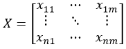
Each row Xr_i in X represents the values of each dimension’s time series at a given time point, and each column Xc_j represents a time series.

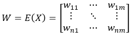
Using a single-dimension anomaly detection algorithm E(…), we calculate the alarm intensity matrix W for each dimension. We know that the elements in W can be greater than 1, and theoretically infinite. To prevent a large value from unduly influencing the overall calculation, and considering that an alarm intensity of 1 already indicates a significant anomaly, we force all elements in W greater than 1 to 1.

w_ij=if(w_ij>1,1,w_ij)

Each time point has a weight sequence, meaning the weights also form a matrix H:

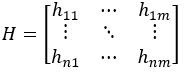
The weight Hr_i at the current time point is calculated using the alarm intensity Wr[-k]_i from a previous interval:

Hr_i=F(Wr[-k]_i)

where F(…) is the method for calculating weights based on the above principle.

Now, let’s examine the specific calculation method for F(…), i.e., how to compute the weight sequence Hr_i for the i-th time point.

Let Z =W[-k]_i

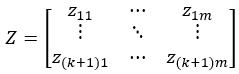
Where z_ij is the alarm intensity of the j-th dimension at the i-th time point in Z.

1. Compute the total alarm intensity SZ:

SZ=[sz₁,sz₂,…,sz_m]

sz_j=sum(Zc_j),j∈[1,m]

Where sz_j is the total alarm intensity of the j-th dimension of SZ.

2. Compute the weight Hr_i at the i-th time point:

Each time point yields a weight sequence SZ.

SZ=[sz₁,sz₂,…,sz_m]

Assume Hr_i=Y

Y=[y₁,y₂,…,y_m]

Where y_j is the weight of the j-th dimensional time series.

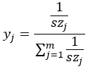
To avoid ‘survivorship bias’, the larger sz_j is, the smaller y_j should be. The weights Y are obtained by taking the reciprocal of the elements in SZ and then applying a linear transformation.

All elements in SZ may be 0, that is, no alarms in any dimension. In this case, we force the weights of each dimension to be equal. It’s also possible that some elements in SZ are 0, that is, sz_j may be 0 and thus have no reciprocal. In this case, we can force its reciprocal to be equal to twice the reciprocal of the largest non-zero element in SZ. Considering these factors, y_j needs to be adjusted:

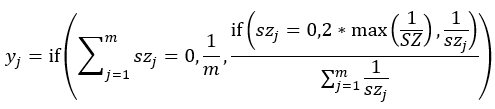
Where 1/SZ represents the reciprocal sequence of the non-zero elements in SZ.

With the weight Hr_i, it is easy to compute the aggregated alarm intensity AW_i:

AW_i=sum(Wr_i **Hr_i)

SPL routine:

	A	B
1	=file(C1).import@tci().(if(~>1,1,~))	/Alarm intensity Xc1 for the first dimension
2	=file(C2).import@tci().(if(~>1,1,~))	/Alarm intensity Xc2 for the second dimension
3	1000	/Learning interval length k
4	[0,0.01,0.1,0.5,1]
5	=to(A3)
6	=A1(A5)	/Learning data for the first dimension
7	=A2(A5)	/Learning data for the second dimension
8	=A6.sum()	/SZ1
9	=A7.sum()	/SZ2
10	=[A8,A9]
11	if A10.sum()==0	=Hri=A10.(1/A10.len())	/Weight Hri when all SZ elements are 0
12	else	=A10.select(~!=0)
13		=B12.max(1/~)
14		=A10.(if(~==0,B13*2,1/~))	/Handle non-zero elements
15		=s=B14.sum(),Hri=B14.(~/s)	/Weight Hri
16	=[A1(A3+1),A2(A3+1)]	/Wri
17	=sum(A16**Hri)	/AWi

Calculation result example:

Alarm intensity graph for two dimensions:

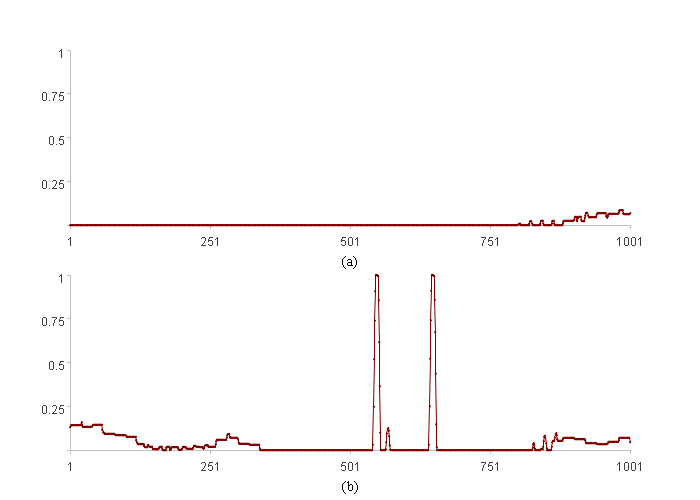
In the graph, both x-axes represent the index, and both y-axes represent the alarm intensity.

Figures (a) and (b) show the alarm intensity trends for the first and second dimensions, respectively. As seen in the figures, within the learning interval ([1, 1000]), the second dimension exhibits more frequent alarms and higher alarm intensity than the first dimension, indicating that its weight should be lower. The weights calculated in the routine matched these expectations, with values of 0.88 and 0.12, respectively.

The aggregated alarm intensity at the final time point (the current time) is 0.065.