The anomaly detection method introduced in the previous section treats ‘clustered’ points as normal and ‘scattered’ points as anomalous. ‘Clustering’ is often irregular; points are considered ‘clustered’ as long as they are close to each other in the multidimensional space. ‘Clustering’ in certain scenarios, however, exhibits strong regularity, as illustrated in the figure below.

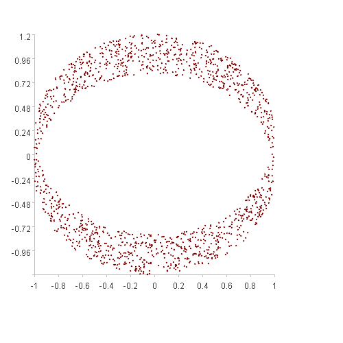
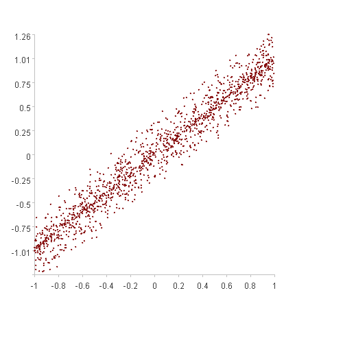
The points in both figures are clustered based on a certain rule, but using the spatial distance method described in the previous section is unlikely to be effective, potentially resulting in many false positives or false negatives.

For such multidimensional time series with recognizable clustering rules, we can compute derived series based on those rules, thereby transforming the problem of multidimensional anomaly detection into a one-dimensional anomaly detection problem on the derived series.

Multidimensional time series X

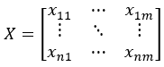
Using a mathematical transformation Dv(…), a one-dimensional time series D is derived:

D=Dv(X,…)

Perform one-dimensional anomaly detection on D to obtain an anomaly score sequence Od:

Od=Sg(D,…)

Let’s illustrate the derivation method using the most common linearly clustered two-dimensional time series as an example.

Two-dimensional time series X:

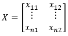
Xc₁ and Xc₂ may be non-linear overall, but within a relatively small interval Xr[-k]_i, they are approximately linear. We can perform the derivation as follows:

1. Within Xr[-k]_i, the coefficients w_i are determined through least-squares fitting.

Let Z=Xr[-k]_i

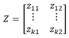
w_i=linefit(Zc₁,Zc₂)

2. Compute the predicted value x’_i2 of x_i2 using w_i and the current point x_i1:

x’_i2=w_i* x_i1

3. The difference between the actual x_i2 and the predicted x’_i2 is the derived value df_i:

df_i=x_i2-x’_i2

The derived series Df is a set of df_i values, with each df_i value corresponding one-to-one with each Xr_i value.

Df=[df₁,df₂,…,df_n]

SPL routine:

	A	B
1	=file(“linedata1.csv”).import@tci()	/First dimension data
2	=file(“linedata2.csv”).import@tci()	/Second dimension data
3	15	/Feature interval k
4	=A1.(~[-A3,-1].(~|1)).to(A3+1,)	/Zc1
5	=A2.(~[-A3,-1].([~])).to(A3+1,)	/Zc2
6	=A4.(linefit(~,A5(#)))	/wi
7	=A1.([~1]).to(A3+1,)	/[xi1,1](excluding the first k points)
8	=A6.(mul(A7(#),~))	/x‘i2 (excluding the first k points)
9	=A2.to(A3+1,)	/xi2 (excluding the first k points)
10	=A9–A8	/Df

A6 is the process of computing w_i using the least squares method.

A8 is the process of computing the predicted value x‘_i2.

Calculation result example:

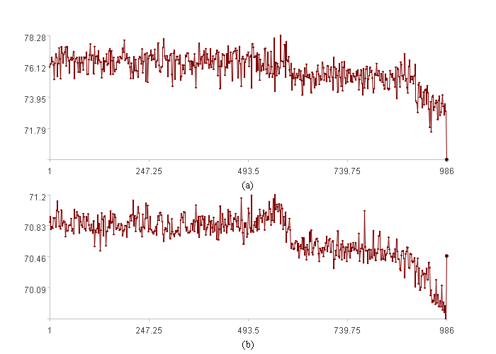
The first figure shows the trend plots of the two-dimensional time series, with the x-axis representing the time series index, the y-axis in (a) representing X_c1, the y-axis in (b) representing X_c2, and the bold points are observation points.

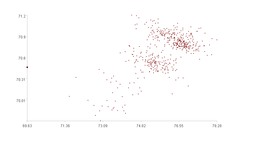
The second figure shows the relationship between the two time series, with the x-axis representing X_c1, the y-axis representing X_c2, and the bold points are observation points.

Observing the second figure, the two series exhibit a linear correlation trend, but the observation points are clearly outside the linearly correlated “cluster” area, and are therefore considered anomalous. Observing the first figure, the curves generally increase or decrease together; however, the observation point exhibits an anomalous behavior: X_c1 decreases while X_c2 increases significantly, which is also considered anomalous.

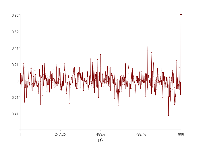
The trend plot of the derived series is shown above. The x-axis represents the time-series index, and the y-axis represents the values of the derived series. The observation points are bolded. Because there are no derived values for the first k points, the derived series contains k fewer points.

Observing the derived series in the figure above, it is found that the observation points exhibit very large derived values. We know that single-dimensional anomaly detection algorithms will identify such extreme values. Looking closer at the figure, all points that are particularly large or particularly small correspond to the anomalous behavior of the original time series.