Although the original values may fluctuate frequently, they generally exhibit a trend. The ‘main line’ is a derived series that describes this trend.

In simple terms, smoothing the original values reveals their trend. The most common smoothing approach is averaging, which, when applied to time series, is moving average.

The main line M of the time series X is calculated as:

m_i=avg(X[-(l+1)]_i+1)

SPL routine:

	A	B	C
1	=data=file(“1Ddata.csv”).import@tci().to(100)		/Time series X
2	=l=5		/Interval l
3	=A1.(if(#<=l,null,(s=~[-l:-1],avg(s))))		/Main line M

The main line M is calculated in cell A3.

Thought: Implement linear weighted moving average (LWMA) and exponential weighted moving average (EWMA) in SPL.

Calculation result example:

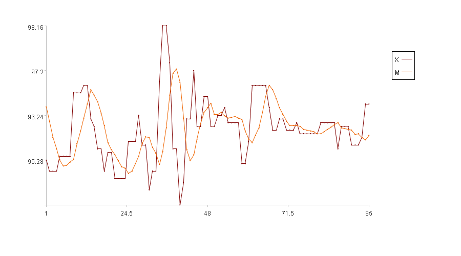
In the figure, the x-axis represents the sequence index, and the y-axis represents the values of the original series X. In the legend, X is the original series and M is the main line. (Because the first five time points have no main line values, the figure only displays the main line values of the subsequent 95 time points).

While calculating the moving average is convenient and it provides good smoothing, it has a key drawback: each point on the main line represents the average of all values within a preceding interval. This inevitably causes the main line to lag behind the original values, that is, when the original values begin to decrease, the main line may remain static, decreasing only after a delay. Consequently, anomaly detection can be delayed, making this method unsuitable for time-critical scenarios.

Let’s consider an alternative method for calculating the main line.

The main line should represent the information of the original values, so it should, in principle, closely approximate these values. Moreover, to ensure smoothness, adjacent points on the main line should also be close. Assuming a main line has been calculated, we define the sum of absolute differences between the main line and the original values as the ‘Original Value Distance’, and the sum of absolute differences between adjacent points on the main line as the ‘Main Line Distance’. A suitable main line should minimize both the Original Value Distance and the Main Line Distance. Therefore, a suitable main line M can be found by minimizing a weighted sum of these distances.

The main line calculated using this method balances the two types of distances, resulting in a minimal delay effect and high timeliness, making it well-suited for time-critical scenarios. However, this method also has a drawback: its computational complexity is considerably higher than that of the moving average, requiring careful consideration in scenarios where computing efficiency is a high priority.

1. Calculating distances

The Main Line Distance, denoted as MD, is the sum of the distances (squared differences) between adjacent points on the main line.

MD=sum(m_i-m_i-1)²

The Original Value Distance, denoted as VD, is the sum of the distances (squared differences) between the main line and the original values:

VD=sum(m_i-x_i)²

2. Minimizing the weighted sum of MD and VD

Define a balancing coefficient, k, to balance the weights of MD and VD. The total distance D is then:

D=VD+k*MD

3. Optimizing m_i to minimize the total distance D

Compute the partial derivative with respect to each m_i:

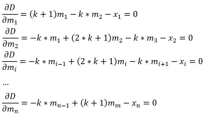
The transformed problem becomes solving a system of multivariate linear equations.

The coefficient matrix is denoted as Cm:

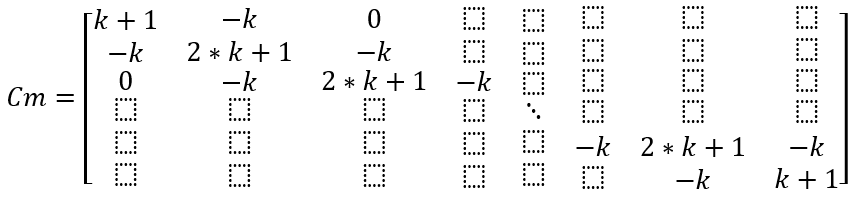
Unspecified entries in the matrix are all 0.

Cm*M=X

Solving the above equation yields the main line M:

M=linefit(Cm,X)

Where linefit() is a function for solving linear equations.

The balancing coefficient k adjusts the weights of the two types of distances. A larger k gives greater weight to MD, resulting in a smoother main line. A smaller k gives greater weight to VD, causing the main line to more closely approximate the original values. When k=0, the main line is exactly the original values. When k=∞, the main line is a constant, equal to the average of the original values.

SPL routine:

	A	B	C
1	=data=file(“1Ddata.csv”).import@tci().to(100)		/Time series X
2	=k=10		/Balancing coefficient k
3	=ln=data.len()		/Sequence length
4	=A1.(if(#==1,[k+1,-k].insert(0,(ln-#-2).(0)), if(#==ln,(#-2).(0).insert(0,[-k,k+1]), (#-2).(0).insert(0,[-k,2*k+1,-k]).insert(0,(ln-#-1).(0)))))		/Coefficient matrix Cm
5	=linefit(A4,A1).conj()		/Calculate main line using least squares method

The coefficient matrix Cm is constructed in cell A4;

The main line sequence M is calculated in cell A5.

Calculation result example:

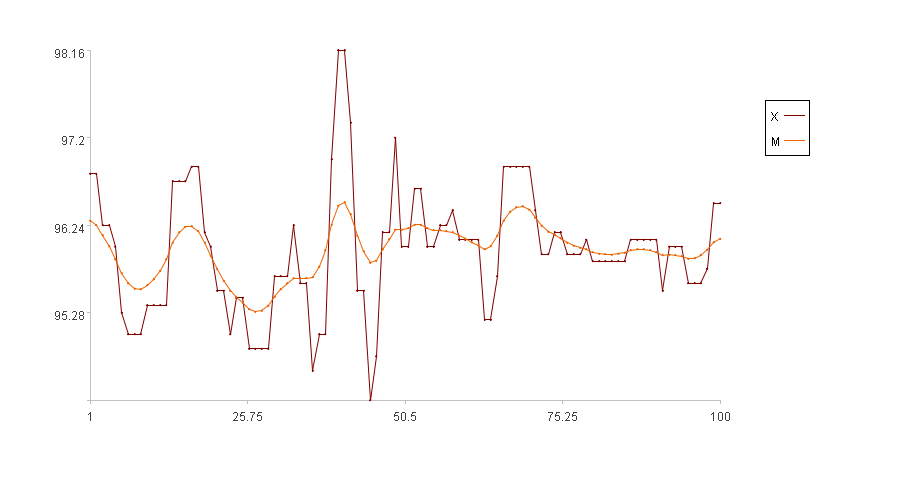
In the figure, the x-axis represents the sequence index, and the y-axis represents the values of the original series X. In the legend, X is the original series and M is the main line.