

2.3 Dispersion
Dispersion is a derived series describing the distribution of the original values.
In statistics, variance is frequently used to measure the degree of dispersion of a set of data. We can also apply variance to calculate dispersion, which we’ll refer to as the ‘variance method’.
The dispersion series S for a time series X is calculated as:
si=sum((xj-a)2)/(n-1),j∈[1,n]
Where n=l+1, which is the length of X[-(l+1)]i+1; xj is the j-th element of X[-(l+1)]i+1; a is the average of the values in X[-(l+1)]i+1.
SPL routine:
| A | B | C | |
|---|---|---|---|
| 1 | =data=file(“1Ddata.csv”).import@tci().to(100) | /Time series X | |
| 2 | =l=5 | /Interval l | |
| 3 | =data.((if(#<=l,null,(s=~[-l:0],var@s(s))))) | /Dispersion S | |
The dispersion series S is calculated in cell A3. The function var@s(…) computes the variance.
Calculation result example:
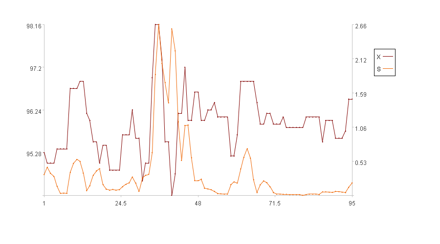
In the figure, the x-axis represents the sequence index, the left y-axis represents the values of the original series X, and the right y-axis represents the values of the dispersion S. In the legend, X is the original series and S is the dispersion. (Because the first five time points have no dispersion, the figure only displays the dispersion for the subsequent 95 time points).
SPL Official Website 👉 https://www.esproc.com
SPL Feedback and Help 👉 https://www.reddit.com/r/esProcSPL
SPL Learning Material 👉 https://c.esproc.com
SPL Source Code and Package 👉 https://github.com/SPLWare/esProc
Discord 👉 https://discord.gg/sxd59A8F2W
Youtube 👉 https://www.youtube.com/@esProc_SPL

