

1.6 Percentage threshold adjustment
Regardless of which of the aforementioned methods is used, the upper threshold tu and the lower threshold td always lie within the learning interval. This presents a problem: when xi exceeds the maximum or falls below the minimum value within the learning interval, xi will inevitably be considered an anomaly.
However, we may sometimes want to avoid regarding xi as an anomaly when it only slightly exceeds the limits. The solution is simple: expand tu and contract td. This is achieved by adjusting the thresholds based on a percentage of the difference between tu and td. Let dst represent the desired percentage of that difference. The adjusted upper threshold tu’ and the adjusted lower threshold td’ are calculated as follows:
tu’=tu+dst*(tu-td)
td’=td-dst*(tu-td)
Theoretically, the range of dst is [-0.5, ∞). However, we typically need to widen the range between tu and td, implying that dst>0. If dst is excessively large, no anomalies will be detected. Therefore, dst is usually kept below 1, with a commonly used range of [0,1].
The method of adjusting thresholds using a percentage of the difference between the upper and lower thresholds is called the Percentage Threshold Adjustment method.
SPL routine:
Time series X is shown below:
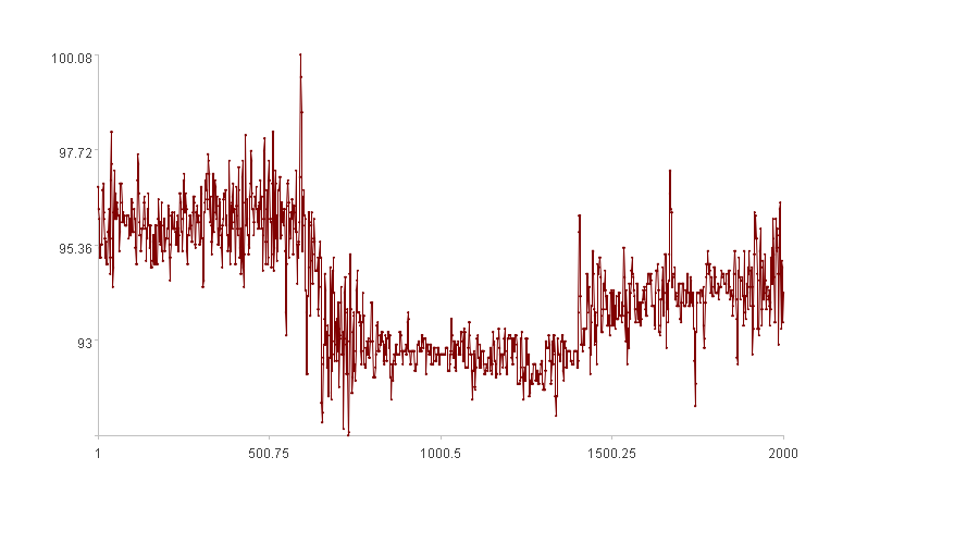
Apply the distance method to X to detect anomalies and calculate the anomaly score for each data point.
SPL routine:
| A | B | |
|---|---|---|
| 1 | =file(C1).import@tci() | /Time series X |
| 2 | 100 | /Learning interval k |
| 3 | 2 | /Radius multiplier |
| 4 | 0 | /dst |
| 5 | =A1.(if(#<=A2,,Threshold(~[-A2:-1],“up”,A3))) | /Upper threshold |
| 6 | =A1.(if(#<=A2,,Threshold(~[-A2:-1],“down”,A3))) | /Lower threshold |
| 7 | =to(A2+1,A1.len()) | /Valid X indices |
| 8 | =A1(A7) | /Valid X |
| 9 | =A5(A7) | /tu |
| 10 | =A6(A7) | /td |
| 11 | =A9.((d=~-A10(#),~+A4*d)) | /tu’ |
| 12 | =A10.((d=A9(#)-~,~-A4*d)) | /td’ |
| 13 | =A8.((a=max(~-A11(#),A12(#)-~,0),b=(A11(#)-A12(#)),if(a==0,0,if(b==0,1,a/b)))) | /Anomaly score Od |
Parameter settings:
Learning interval k=100;
Radius multiplier for the distance method: n=2;
Threshold difference percentage dst=0.
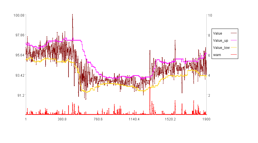
In the figure, Value represents the X values, Value_up the tu sequence, Value_low the td sequence, and warn the anomaly score Od. Since the first 100 points comprise the learning interval, they have no associated anomaly scores. Consequently, the time series in the figure has a length of 1900.
The figure shows that there are too many anomalous time points. Intuitively, detecting so many anomalies seems unnecessary. Adjusting dst can prevent the detection of points with low anomaly scores.
Set dst=0.3
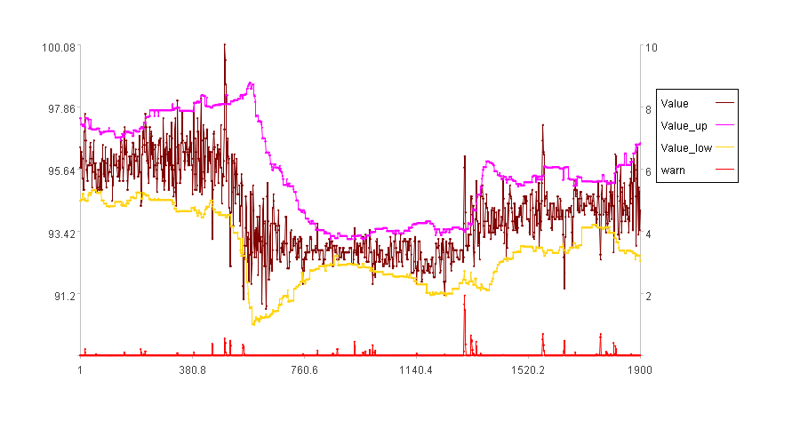
With dst set to 0.3, tu increases and td decreases, making the anomaly detection less sensitive.
SPL Official Website 👉 https://www.esproc.com
SPL Feedback and Help 👉 https://www.reddit.com/r/esProcSPL
SPL Learning Material 👉 https://c.esproc.com
SPL Source Code and Package 👉 https://github.com/SPLWare/esProc
Discord 👉 https://discord.gg/sxd59A8F2W
Youtube 👉 https://www.youtube.com/@esProc_SPL

