

SPL Quantitative Trading Practice Series: Turtle Trading Strategy
The specific rule of Turtle Trading Strategy is like this: buy a stock when the price breaks above the last N-day (usually N is 20) high and sell it when the price falls below the last N-day low. These peaks and lows construct a channel that called Donchian Channel.
Generate buy/sell signals (signal) in this manner: set buy signal (1) when the price exceeds the Donchian Channel upper band, sell signal (-1) when it is below the lower band, and no action (0) at all other times.
Place a buy order if there is a buy signal and no positions are held; place a sell order if there is a sell signal and positions are currently held. And generate order signals (flag) according to that: make a purchase when flag=1, perform selling when flag=-1, and give no action when flag=0.
Take stock code 300750 as an example, the trading period is from January 1, 2020 to March 6, 2024. During this period, 300750 underwent corporate actions such as dividend distribution and stock splits, requiring the stock price to be adjusted for backtesting. Typically, backward-adjusted prices are used for backtesting (See Adjusted Stock Prices for backward adjustment method).
SPL code:
| A | |
|---|---|
| 1 | =file(“daily/300750.csv”).import@tc() |
| 2 | =A1.select(trade_date>=20200101&&trade_date<=20240306) |
| 3 | =A2.derive(if(#>1, close/ pre_close *factor[-1], close/pre_close):factor) |
| 4 | =hfq_fst=A3(1),A3.derive(round(factor/hfq_fst.factor*hfq_fst.close,2): hfq_close) |
| 5 | =ps=0 |
| 6 | =A4.new(ts_code,trade_date,hfq_close,if(#==1,hfq_close,hfq_close[-20:-1].max()):taq_up,if(#==1,hfq_close,hfq_close[-20:-1].min()):taq_down,if(#>20&&hfq_close>taq_up,1,if(#>20&&hfq_close<taq_down,-1,0)):signal,if(ps==0&&signal==1,(ps=1,1),if(ps!=0&&signal==-1,(ps=0,-1),0)):flag,if(flag!=0,100,0):shares) |
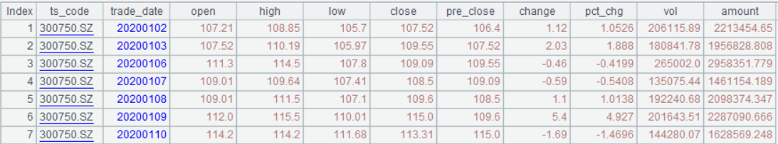
A2: Below is part of the table recording stock market data from January 1, 2020 to March 6, 2024:
A3: Generate price adjustment factor.
A4: Compute backward adjusted price.
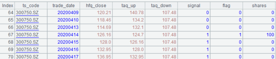
A6: Generate Donchian Channel (taq_up: upper band; taq_down: lower band), buy/sell signals, and order signals (flag); and define the number of shares involved in each transaction as 100.
Below shows part of the result set:
SPL offers operator [] to obtain elements before or after the current one. It gets continuous elements before the current one when enclosing negative numbers, and ones after the current element when using positive numbers. close[-20:-1], for example, represents a set of close field members from the 20th to the first before the current one. Python uses shift(1).rolling(20) to express the same concept, where shift(1) specifies the offset value and rolling(20) packages the 20 members before the current one as a difficult to understand object. SPL, by contrast, produces clear and simple code.
In expression A4.new(…), each newly-generated field is useful in the directly subsequent computation. taq_up and taq_down are used for computing signal, and signal is used to compute flag. Python cannot do this, but can only compute values of each field one by one.
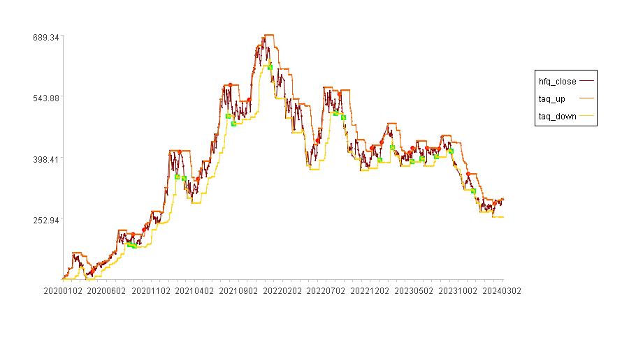
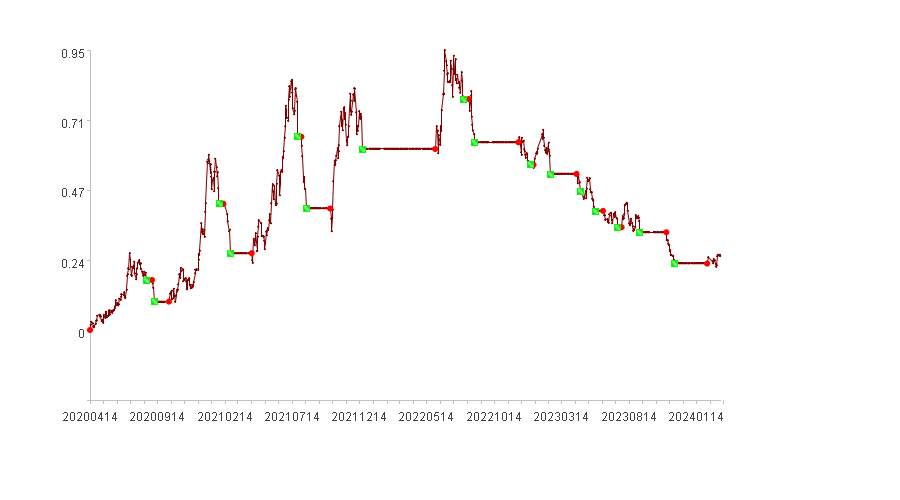
According to A6’s data, we can plot the backward-adjusted stock price trend, Donchian channel and buy/sell points. But first, we need to convert trade_date values to date type. Then plot trade_date the horizontal axis and stock price the vertical axis, and draw points when flag=1 as buy points (highlighted in red dots) and points when flag=-1 as sell points (highlighted in green squares).
Below is the buy/sell run chart:
According to the backtesting routine explained in SPL Quantitative Practice Series: Backtesting Routine, find A6’s records where flag isn’t equal to 0 – which are trade_date values input for backtesting. Here is the result set:
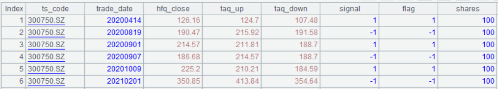
Then set the ending date as 20240306 to perform the backtesting.
Below is RoR run chart:
In the above run chart, the vertical axis displays RoRs, red dots are buy points, and green squares are sell points.
The following table lists backtested indicators:
| Indicators | Value |
|---|---|
| Cumulative rate of return | 25.05% |
| Annualized rate of return | 6.14% |
| Annual volatility | 35.77% |
| Sharpe ratio | 0.09 |
| Maximum drawdown | 37.68% |
| Cash invested | 37916.59 |
| Total assets | 47416.59 |
| Stock holding ratio | 62.74% |
| Profits count | 5 |
| Losses count | 11 |
SPL Official Website 👉 https://www.esproc.com
SPL Feedback and Help 👉 https://www.reddit.com/r/esProcSPL
SPL Learning Material 👉 https://c.esproc.com
SPL Source Code and Package 👉 https://github.com/SPLWare/esProc
Discord 👉 https://discord.gg/sxd59A8F2W
Youtube 👉 https://www.youtube.com/@esProc_SPL


Chinese version