6.1 Data information

Start esProc and run createEventsAndUsers.splx, you can get the following two tables (can also modify the start and end dates and daily data amount according to comments in the code of the splx file):

Ecommerce events table (events.csv):

Field	Description
eventID	Event ID, whose values are sequence numbers starting from 1
userID	User ID
eTime	The datetime when an ecommerce event happens
eType	Ecommerce event type, whose value is login, viewProduct, placeOrder, or completePayment

Records are ordered by both eTime field and eventID field. As data are appended in chronological order, they are always ordered by eTime; as eventID is the sequence number, they are naturally ordered.

Users table (user.csv):

Field	Description
userID	User ID, whose values are sequence numbers starting from 1
userName	User name
city	The city where user is based

Relationship between the tables:

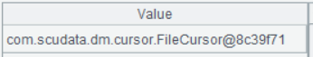
6.2 Select all records of events happened in 2024 National Day holiday

The events table is too large to fit into the memory, and cursor is needed. SPL offers file cursor, on which filtering, grouping, aggregation and other operations can be performed.

	A
1	=file(“events.csv”).iselect@tc(date("2024-10-01"):datetime("2024-10-07 23:59:59"),eTime ; userID,eTime,eType)

A1 Since the events table is ordered chronologically, iselect() function is used to directly perform filtering on the data file according to time, making it possible to use binary search to increase retrieval efficiency by skipping records not meeting the filtering condition.

Parameters before the semicolon mean selecting records whose eTime values are within the closed interval date("2024-10-01"):datetime("2024-10-07 23:59:59").

Parameters (userID, eTime, eType)after the semicolon are fields to be selected. The other fields will not be selected and memory usage will become less. iselect() function returns a cursor on which the next step of computations can be directly performed. If data needs to be exported, just perform fetch() operation.

Below is result of executing A1’s statement:

The above screenshot shows that the result A1 returns is a cursor.

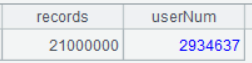
6.3 Count event records and users in 2024 National Day holiday

	A
1	=file(“events.csv”).iselect@tc(date(“2024-10-01”):datetime(“2024-10-07 23:59:59”),eTime ; userID,eTime,eType)
2	=A1.groups(**;**count(1):records,icount(userID):userNum)

A2 Perform grouping & aggregation. groups() function performs operations directly on the cursor and returns the aggregation result. Note that when there isn’t the grouping expression written before the semicolon, the function performs aggregation on the whole set.

Below is result of executing A2’s statement:

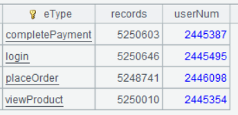
6.4 Count event records and users in 2024 National Day holiday by event type

	A
1	=file(“events.csv”).iselect@tc(date(“2024-10-01”):datetime(“2024-10-07 23:59:59”),eTime;userID,eTime,eType)
2	=A1.groups(eType;count(1):records,icount(userID):userNum)

Below is result of executing A2’s statement:

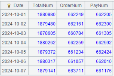
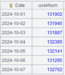
6.5 Count the total number of users, users who placed an order, and users who paid in each day of 2024 National Day holiday

	A
1	=file(“events.csv”).iselect@tc(date(“2024-10-01”):datetime(“2024-10-07 23:59:59”),eTime;userID,eTime,eType)
2	=A1.group(date(eTime):Date; ~.icount(userID):TotalNum, ~.select(eType==“placeOrder”).icount(userID):OrderNum, ~.select(eType==“completePayment”).icount(userID):PayNum)
3	=A2.fetch()

A2 Perform grouping operation on A1’s cursor. group()function will retain the grouped subsets. In ~.icount(userID), ~ represents the current subset; the whole expression counts distinct userIDs in the current subset. ~.select(eType==“placeOrder”).icount(userID) first performs filtering on the current subset to get records whose eType value is placeOrder and then counts distinct userIDs in the subset.

cs.group() function still returns a cursor. Below is result of executing A2’s statement:

A3 fetches result data from A2’s cursor.

Below is result of executing A3’s statement:

6.6 Count daily number of Beijing users who placed an order in 2024 National Day holiday

	A
1	=file(“events.csv”).iselect@tc(date(“2024-10-01”):datetime(“2024-10-07 23:59:59”),eTime;userID,eTime,eType)
2	=file(“user.csv”).cursor@tc(userID,city).select(city==“Beijing”).fetch()
3	=A1.select(eType==“placeOrder”).join@i(userID,A2:userID)
4	=A3.groups(date(eTime):Date;icount(userID):userNum)

A2 The users table also has a large amount of data. Here only records of Beijing region need to be retrieved, so we can use the cursor for data retrieval, perform filtering on the cursor, and then perform fetch(). This way user records of non-Beijing region will not occupy the memory space.

A3 Select records where users placed an order from A1 and perform join between them and A2. @i option means deleting A2’s records that do not have their matches in A1 and only retaining those that have a match (to retain A2’s records that do not have their matches only and delete those that have a match, such as performing aggregation on records of users who are not in Beijing region, we can replace @i option with @d option while the rest of the statement remains unchanged). Since A1 is a cursor, A3 still returns a cursor.

A4 Perform grouping & aggregation on A3.

Below is result of executing A4’s statement:

Learning point: Filtering before join

In the preceding example, filtering operation is first performed on the two objects to be joined respectively before the join, reducing the number of comparisons and thus increasing efficiency.

6.7 Split events table into multiple tables by month and sort each smaller table by userID

As the events table is too large to fit into the memory, the cursor is needed to perform sorting on it:

	A
1	=file(“events.csv”).iselect@tc(date(“2024-10-01”):datetime(“2024-10-31 23:59:59”),eTime).sortx(userID)
2	=file(“events202410.csv”).export@tc(A1)
3	=file(“events.csv”).iselect@tc(date(“2024-11-01”):datetime(“2024-11-30 23:59:59”),eTime).sortx(userID)
4	=file(“events202411.csv”).export@tc(A3)
5	=file(“events.csv”).iselect@tc(date(“2024-12-01”):datetime(“2024-12-31 23:59:59”),eTime).sortx(userID)
6	=file(“events202412.csv”).export@tc(A5)

A1 sortx() function is specially used to sort a cursor. Here its parameter userID is the sorting field. The function also returns a cursor.

A2 Retrieve data from A1’s cursor and write them directly to events202410.csv. export()has the same rule in using options as import(); the former is the inverse operation of the latter.

Learning point: Differences between sort()and sortx()

1.sort()

Characteristics:

• Execute instantly: Sorting is directly performed on the current table sequence (record sequence) when sort() is called, and a new ordered result is generated.
• Perform in-memory sorting: Sort small and medium-sized datasets in the memory.
• Return a new sequence: The original sequence remains unchanged, and the function returns the new sequence after sorting.

Application scenarios:

The function is suitable for dealing with scenarios where datasets can be completely loaded into the memory and where the sorting result needs to be directly obtained.

2.sortx()

Characteristics:

• Execute instantly: Save sorting result in one or more temporary files and return a merging cursor of these files.
• Perform sorting on external storage: Sort large datasets that cannot wholly loaded into the memory by handling them through temporary files.
• Return a cursor: Return cursor of the sorting result, which can be exported or further computed.

Application scenarios:

The function is suitable for dealing with scenarios where datasets cannot be completely loaded into the memory or where delayed operations (such as stream processing) are also involved.

6.8 Count orders placed per user in the specified months respectively

Implement the following summarization tasks:

1. Count users who placed an order in October; count orders placed in October and November respectively.

2. Find users who placed an order in both October and November; count orders placed in October and November respectively.

3. Count each user’s orders placed in October and November respectively.

Step 1: Generate cursors

	A
1	=file(“events202410.csv”).cursor@tc()
2	=file(“events202411.csv”).cursor@tc()

Step 2: Compute the number of orders in October and November respectively.

	A
3	=A1.select(eType==“placeOrder”).group(userID;~.count(1):10Num)
4	=A2.select(eType==“placeOrder”).group(userID;~.count(1):11Num)

A3 Since A1 is a cursor, select()function returns a cursor and group() function also returns cursor.

Step 3: Perform join

1. Get records of users who placed an order in October; count orders placed in October and November respectively.

	A
5	=joinx@1(A3:oct,userID;A4:nov,userID)
6	=A5.new(oct.userID,oct.10Num,nov.11Num)
7	=file(“result.csv”).export@tc(A6)

A5 joinx@1 means left join. joinx() function is intended to perform the join between two or more cursors. It requires that each of the cursors to be joined be ordered by the join field. The function uses same parameter rules as join() does.

A6 Same as join(), joinx()’s joining result is a referencing field. It needs another new() operation to generate the result table sequence. A6 is still a cursor.

A7 Export result to a file. As the result set is too large to fit into the memory, we can directly export data in the cursor to a file.

2. Get records of users who placed an order in both October and November; and count orders placed in October and November respectively.

	A
5	=joinx(A3:oct,userID;A4:nov,userID)
6	=A5.new(oct.userID,oct.10Num,nov.11Num)
7	=file(“result.csv”).export@tc(A6)

A5 joinx() means inner join.

3. Count each user’s orders placed in October and November respectively.

	A
5	=joinx@f(A3:oct,userID;A4:nov,userID)
6	=A5.new(oct.userID,oct.10Num,nov.11Num)
7	=file(“result.csv”).export@tc(A6)

A5 joinx@f means full join.

Learning point: Differences between join()and joinx()

1.join()

Characteristics:

• Execute immediately: The join operation is directly executed when join() is called, and a new result table sequence is generated.
• Perform in-memory join: Perform a join between small and medium-sized datasets in the memory.
• Return the whole result: Load the joining result set all into the memory.
• Flexible syntax: Support multiple join types (including inner join, left join and full join).
• Allow unordered data: Do not require data to be ordered by the join field.

Application scenarios:

• Where datasets can be wholly loaded into the memory.
• Where the joining result needs to be directly obtained

2.joinx()

Characteristics:

• Delayed execution: joinx()only generates a joining cursor without executing the computation immediately. The actual join operation will be postponed until the subsequent traversal or aggregation starts to execute.
• Perform external memory join: Support join between large datasets to handle data exceeding memory capacity.
• Lazy evaluation: Suitable for stream processing and can work with the other functions (such as groups() and select()).
• Return a cursor: Do not directly return the whole result, it returns an iterable cursor object instead.
• Required ordered data: Require data to be ordered by the join field.

Application scenarios:

• Where datasets cannot be wholly loaded into the memory.
• Where delayed operations (such as stream processing) are also involved.