We have already implemented a method for discovering single-shape curve segments. Sometimes, we also need to discover composite shapes where two or more shapes appear consecutively, such as a curve that first falls then stabilizes, or one that first rises, stabilizes, and then falls, and so on.

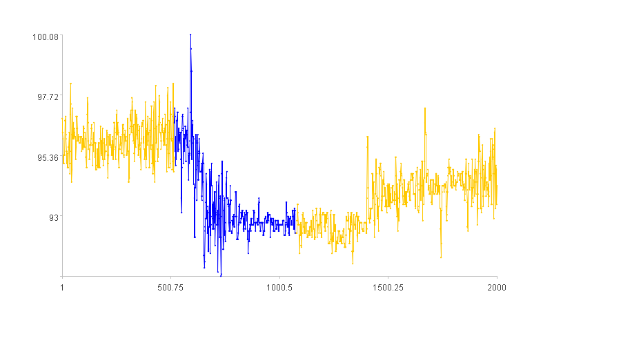
Using the previous time series, let’s find the curve segments that first fall then stabilize. The blue curves in the figure below indicate the approximate locations of these segments.

Now let’s describe how to discover consecutive multi-shape curve segments:

1. Find the curve segment indices for each shape using the single-shape curve segment discovery method:

Id⁽¹⁾=H(arg₁)=[Id⁽¹⁾(1), Id⁽¹⁾ (2),…, Id⁽¹⁾ (p₁)]

Id⁽²⁾=H(arg₂)=[Id⁽²⁾(1), Id⁽²⁾ (2),…, Id⁽²⁾ (p₂)]

…

Id^(k)=H(arg_k)=[Id^(k)(1), Id^(k) (2),…, Id^(k) (p_k)]

Ids=[ Id⁽¹⁾(1), Id⁽¹⁾ (2),…, Id⁽¹⁾ (p₁), Id⁽²⁾ (1),…, Id⁽²⁾ (p₂),…, Id^(k)(1),…, Id^(k) (p_k)]

Where Id⁽ⁱ⁾ is the index set of the i-th shape, Id⁽ⁱ⁾ (j) is the j-th segment of Id⁽ⁱ⁾, H(…) is the function for discovering single-shape curve segments, and arg_i is the parameter for the i-th shape.

2. Sort Ids by index. Let Idst denote the sorted results:

Idst=Ids.sort(~(1))

Where Idst is the index set sorted based on the first element of each Id⁽ⁱ⁾ (j).

3. Find consecutive shape indices in Idst that match the desired shape order and are not too far apart. Let Idst’ denote the found indices:

Idst’₁=[Id⁽¹⁾(s₁), Id⁽²⁾(t₁),…, Id^(k)(u₁)]

Idst’₂=[Id⁽¹⁾(s₂), Id⁽²⁾(t₂),…, Id^(k)(u₂)]

…

Idst’_v=[Id⁽¹⁾(s₂), Id⁽²⁾(t₂),…, Id^(k)(u₂)]

Where Idst’_i is the index set of the i-th consecutive shape curve segment. Each segment is the index set of k shapes, and the indices of adjacent shapes are not too far apart. That is, the last index of one shape and the first index of the next shape are close. Taking the index set of the first consecutive shape segment as an example:

Id⁽²⁾(t₁)(1)-Id⁽¹⁾(s₁)(-1)<ε

Id⁽²⁾(t₁)(1) is the first index of the t₁-th segment of the second shape, Id⁽¹⁾(s₁).m(-1) is the last index of the s₁-th segment of the first shape, and ε is a relatively small value that can be used as a parameter to ensure that the two shapes are adjacent on the time series X.

4. Extract time series data based on the consecutive shape indices

Since the indices of consecutive shapes are expected to be sequential, the index range for the consecutive shape curve segment is defined from the first index of the first shape to the last index of the k-th shape:

sp_i=X(to(Id⁽¹⁾(s_i)(1), Id^(k)(u_i).m(-1)))

sp_i is the i-th segment of consecutive shape, Id⁽¹⁾(s_i)(1) is the first index of the i-th segment of the first shape, and Id^(k)(u_i).m(-1) is the last index of the i-th segment of the k-th shape.

SPL routine:

The time series data remains unchanged. Discover the curve segments that first fall then stabilize.

We need to fit the main line M and calculate the rise/fall index L.

Parameter settings:

Let K’ denote the observation level:

K’=600

Two sets of parameters are required for the two shapes:

Let Nm₁ denote the combination of falling segment feature index names:

Nm₁=[“L”]

Let Nm₂ denote the combination of stable segment feature index names:

Nm₂=[“L”]

Let Ag₁ denote the value range of the falling segment:

Ag₁=[[-1,-0.1]]

Let Ag₂ denote the value range of the stable segment:

Ag₂=[[-0.1,0.1]]

Let dut₁~ ~denote the shape length range of the falling segment:

dut₁=[100,10000]

Let dut₂ denote the shape length range of the stable segment:

dut₂=[100,10000]

Let ε denote the interval between two segments:

ε=180

SPL routine:

	A	B
1	=file(“1Ddata.csv”).import@tc()	/Table sequence containing time series X
2	600	/K’
3	[L]	/Nm1
4	[[-1,-0.1]]	/Ag1
5	[100,10000]	/dut1
6	[L]	/Nm2
7	[[-0.1,0.1]]	/Ag2
8	[100,10000]	/dut2
9	180	/ε
10	=A1.(Value)	/Time series X
11	=2*power(4,lg(A2/15,2)-1)	/Balancing coefficient K
12	=fit_main(A10,A11)	/Main line M
13	=A2/40	/Index interval k
14	=Lift(A12,A13)	Rise-fall index L
15	=[A14.min(),A14.max()]	/Min & max of L
16	=[A15]	/Min & max of feature index
17	=A1.derive(A14(#):L)	/Table sequence T
18	=A4.((idx=#,~.(arg_throw(~,A16(idx)(2),A16(idx)(1)))))	//Falling segment parameter projection
19	=A3.(~/“>=”/“number(”/$[A18(]/#/$[)(1)]/“)”/“&&”/~/“<=”/“number(”/$[A18(]/#/$[)(2)]/“)”).concat(“&&”)	/Falling segment filtering criteria
20	=A17.pselect@a(eval(A19))
21	=A20.group@u(~-#)
22	=A21.select(~.len()>=A5(1)&&~.len()<=A5(2))	/Falling segment index combination Id(1)
23	=A7.((idx=#,~.(arg_throw(~,A16(idx)(2),A16(idx)(1)))))	/Stable segment parameter projection
24	=A6.(~/“>=”/“number(”/$[A23(]/#/$[)(1)]/“)”/“&&”/~/“<=”/“number(”/$[A23(]/#/$[)(2)]/“)”).concat(“&&”)	/Stable segment filtering criteria
25	=A17.pselect@a(eval(A24))
26	=A25.group@u(~-#)
27	=A26.select(~.len()>=A8(1)&&~.len()<=A8(2))	/Stable segment index combination Id(2)
28	=[A22,A27]	/Ids
29	=A28.conj((idx=#,~.new(~:seq,idx:seq_idx)))	/Indices of curve segments with different shapes
30	=A29.sort(seq)	/Sorted Idst
31	=A30.group@u(seq_idx-#)	/Adjacent grouping
32	=A31.select(~.len()==A28.len()&&(ss=~.(seq),ss(2)(1)-ss(1).m(-1)<=A9))	/Filter Idst’ for groups with sufficiently small intervals
33	=A32.((sq=~.(seq).conj(),to(sq.~,sq.m(-1))))	/Curve segments meeting the requirements
34	=A33.(A10(~))	/Specified shape Sp

Calculation result example:

The discovered consecutive shapes meet expectations.