1. Filtering for curve segments with values between [90, 95]

No need to calculate feature indices or project parameters.

Parameter settings:

Let Nm denote the combination of feature index names:

Nm=[“Value”]

Let Ag denote the range of values:

Ag=[[90,95]]

Let dut denote the shape length range:

dut=[100,10000]

SPL routine:

	A	B
1	=file(“1Ddata.csv”).import@tc()	/Table sequence containing time series X
2	[Value]	/Nm
3	[[90,95]]	/Ag
4	[100,10000]	/dut
5	=A2.(~/“>=”/“number(”/$[A3(]/#/$[)(1)]/“)”/“&&”/~/“<=”/“number(”/$[A3(]/#/$[)(2)]/“)”).concat(“&&”)	/Feature index filtering condition
6	=A1.pselect@a(eval(A5))	/Feature index indices Id
7	=A6.group@u(~-#)	/Adjacent indices form a segment Ids
8	=A7.select(~.len()>=A4(1)&&~.len()<=A4(2))	/Filter Ids’ by length
9	=A1.(Value)	/Time series X
10	=A8.(A9(~))	/Specified shape Sp

Calculation result example:

Time series X:

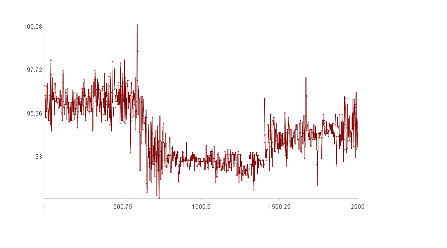
The x-axis represents the index, and the y-axis represents the values of X.

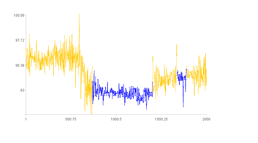
The blue segments in the figure represent the discovered shapes.

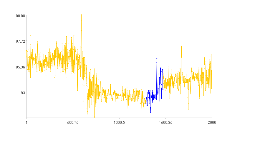
2. Rising curve segments

The rise-fall index L needs to be used. Before calculating L, the main line M needs to be fitted. In addition, parameter projection is required.

Parameter settings:

Let K’ denote the observation level:

K’=600

Let Nm denote the combination of feature index names:

Nm=[“L”]

Let Ag denote the range of values:

Ag=[[0.1,1]]

Let dut denote the shape length range:

dut=[100,10000]

SPL routine:

	A	B
1	=file(“1Ddata.csv”).import@tc()	/Table sequence containing time series X
2	600	/K’
3	[L]	/Nm
4	[[0.1,1]]	/Ag
5	[100,10000]	/dut
6	=A1.(Value)	/Time series X
7	=2*power(4,lg(A2/15,2)-1)	/Balancing coefficient K
8	=fit_main(A6,A7)	/Main line M
9	=A2/40	/Index interval k
10	=Lift(A8,A9)	/Rise-fall index L
11	=[A10.min(),A10.max()]	/Min & max of feature index
12	=[A11]
13	=A4.((idx=#,~.(arg_throw(~,A12(idx)(2),A12(idx)(1)))))	/Parameter projection
14	=A1.derive(A10(#):L)	/Table sequence T
15	=A3.(~/“>=”/“number(”/$[A13(]/#/$[)(1)]/“)”/“&&”/~/“<=”/“number(”/$[A13(]/#/$[)(2)]/“)”).concat(“&&”)	/Feature index filtering condition
16	=A14.pselect@a(eval(A15))	/Feature index indices Id
17	=A16.group@u(~-#)	/Adjacent indices form a segment Ids
18	=A17.select(~.len()>=A5(1)&&~.len()<=A5(2))	/Filter Ids’ by length
19	=A18.(A6(~))	/Specified shape Sp

Calculation result example:

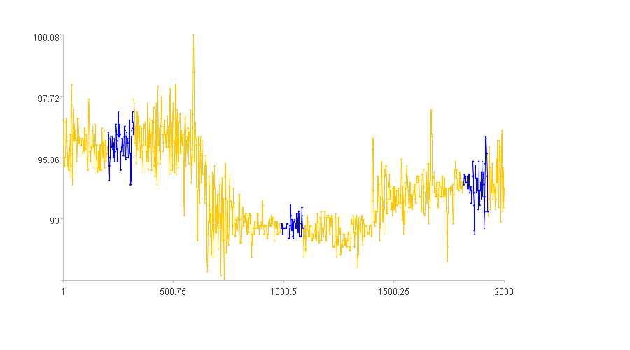
3. Curve segments with high oscillation frequency

The frequency index Vf needs to be used. Before calculating Vf, the main line M and fluctuation curve Wv need to be fitted. In addition, parameter projection is required.

Parameter settings:

Let K’ denote the observation level:

K’=600

Let Nm denote the combination of feature index names:

Nm=[“L”]

Let Ag denote the range of values:

Ag=[[0.1,1]]

Let dut denote the shape length range:

dut=[100,10000]

SPL routine:

	A	B
1	=file(“1Ddata.csv”).import@tc()	/Table sequence containing time series X
2	600	/K’
3	[Vf]	/Nm
4	[[0,1]]	/Ag
5	[100,10000]	/dut
6	=A1.(Value)	/Time series X
7	=2*power(4,lg(A2/15,2)-1)	/Balancing coefficient K
8	=fit_main(A6,A7)	/Main line M
9	=A2/40	/Index interval k
10	=A6–A8	/Fluctuation curve Wv
11	=VFre(A10,A9)	/Frequency index Vf
12	=[A11.min(),A11.max()]	/Min & max of feature index
13	=[A12]
14	=A4.((idx=#,~.(arg_throw(~,A13(idx)(2),A13(idx)(1)))))	/Parameter projection
15	=A1.derive(A11(#):Vf)	/Table sequence T
16	=A3.(~/“>=”/“number(”/$[A14(]/#/$[)(1)]/“)”/“&&”/~/“<=”/“number(”/$[A14(]/#/$[)(2)]/“)”).concat(“&&”)	/Feature index filtering condition
17	=A15.pselect@a(eval(A16))	/Feature index indices Id
18	=A17.group@u(~-#)	/Adjacent indices form a segment Ids
19	=A18.select(~.len()>=A5(1)&&~.len()<=A5(2))	/Filter Ids’ by length
20	=A19.(A6(~))	/Specified shape Sp

Calculation result example:

4. Curve segments exhibiting oscillating divergence

The amplitude rise/fall index VaL and frequency rise/fall index VfL need to be used. Before calculating them, the main line M, fluctuation curve Wv, amplitude index Va, frequency index Vf, amplitude main line VaM, and frequency main line VfM need to be fitted. In addition, parameter projection is required.

Parameter settings:

Let K’ denote the observation level:

K’=600

Let Nm denote the combination of feature index names:

Nm=[“VaL”, “VfL”]

Let Ag denote the range of values:

Ag=[[0,1],[-0.5,1]]

Let dut denote the shape length range:

dut=[100,10000]

SPL routine:

	A	B
1	=file(“1Ddata.csv”).import@tc()	/Table sequence containing time series X
2	600	/K’
3	[VaL, VfL]	/Nm
4	[[0,1],[-0.5,1]]	/Ag
5	[100,10000]	/dut
6	=A1.(Value)	/Time series X
7	=2*power(4,lg(A2/15,2)-1)	/Balance coefficient K
8	=fit_main(A6,A7)	/Main line M
9	=A2/40	/Index interval k
10	=A6–A8	/Fluctuation curve Wv
11	=Amplitude(A10,A9)	/Amplitude Index Va
12	=fit_main(A11,A7)	/Amplitude main line VaM
13	=Lift(A12,A9)	/Amplitude rise/fall index VaL
14	=VFre(A10,A9)	/Frequency Index Vf
15	=fit_main(A14,A7)	/Frequency main line VfM
16	=Lift(A15,A9)	/Frequency rise/fall index VfL
17	=[A13.min(),A13.max()]	/Min & max of VaL
18	=[A16.min(),A16.max()]	/Min & max of VfL
19	=[A17,A18]	/Min & max of feature index
20	=A4.((idx=#,~.(arg_throw(~,A19(idx)(2),A19(idx)(1)))))	/Parameter projection
21	=A1.derive(A13(#):VaL,A16(#):VfL)	/Table sequence T
22	=A3.(~/“>=”/“number(”/$[A20(]/#/$[)(1)]/“)”/“&&”/~/“<=”/“number(”/$[A20(]/#/$[)(2)]/“)”).concat(“&&”)	/Feature index filtering condition
23	=A21.pselect@a(eval(A22))	/Feature index indices Id
24	=A23.group@u(~-#)	/Adjacent indices form a segment Ids
25	=A24.select(~.len()>=A5(1)&&~.len()<=A5(2))	/Filter Ids’ by length
26	=A25.(A6(~))	/Specified shape Sp

Calculation result example: