

1.7 Channel threshold adjustment
While the percentage threshold adjustment method works well for most data, it is ineffective for some specific data, such as the following time series:
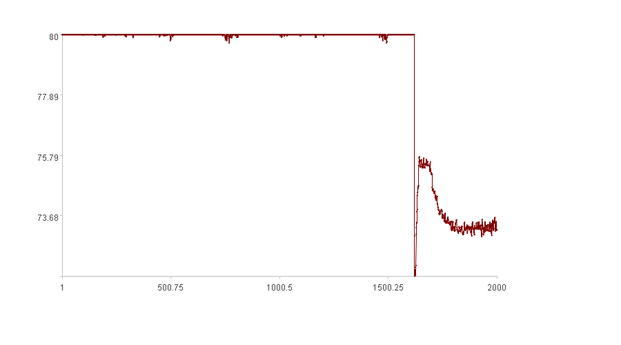
The figure shows that the time series data fluctuates around 80 in the first half, then suddenly drops and stabilizes at around 73 after a transition. Intuitively, this transition period is considered anomalous, while the remaining periods can be regarded as normal.
First, detect anomalies using the original parameters:
Learning interval k=100;
Radius multiplier for the distance method n=2;
Threshold difference percentage dst=0.
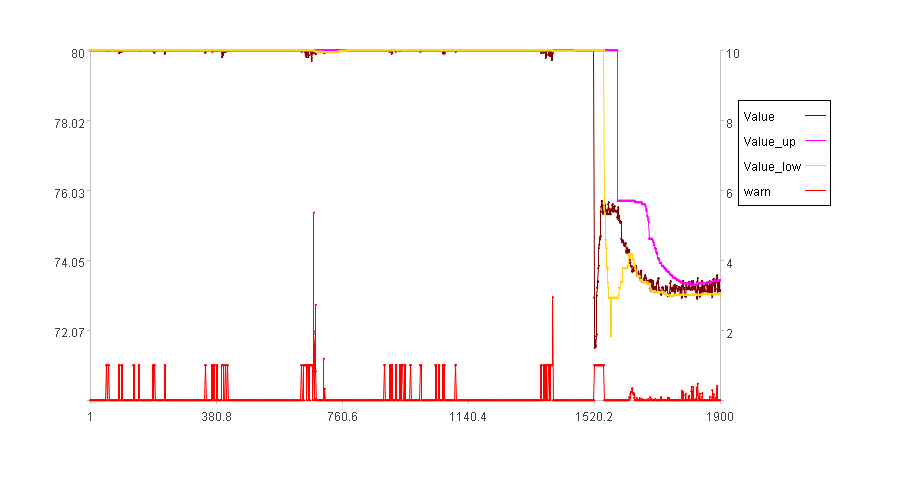
The detected anomalies are consistent with the algorithm’s logic; because the abrupt changes around 80 are indeed infrequent, they can be considered anomalies. However, in comparison to the magnitude of change during the transition period, these variations are insignificant and might be viewed as normal.
Observing tu and td, we find they differ little, or are even equal, in the first half of the time series. Therefore, the percentage threshold adjustment method is ineffective at adjusting the anomaly score during this period.
The following figure shows the anomaly detection results with dst=0.3:
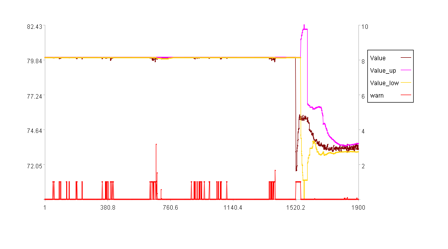
It can be observed that dst has almost no effect. So, how do we deal with this kind of data?
For this type of data, we permit the values of time series X to vary within a defined range; any variations within that range are considered normal. As illustrated above, we permit the data to vary by no more than 0.5. Think of it as a ‘pipe’: data within this ‘pipe’ of a certain width is deemed normal. We refer to this ‘pipe’ as a channel, denoted by ch. The method of adjusting thresholds using a channel is called the Channel Threshold Adjustment method.
The channel threshold adjustment method is also straightforward: When xi is greater than tu and td+ch is also greater than tu, then tu is adjusted to tu’=td+ch; when xi is less than td and tu-ch is also less than td, td is adjusted to td’=tu-ch.
tu’=if(xi>tu&&td+ch>tu, td+ch,tu)
td’=if(xi<td&&tu-ch<td, tu-ch,td)
This ensures that all values of xi is considered normal within the channel ch.
SPL routine:
| A | B | |
|---|---|---|
| 1 | =file(C1).import@tci() | /Time series X |
| 2 | 100 | /Learning interval k |
| 3 | 2 | /Radius multiplier |
| 4 | 0.5 | /ch |
| 5 | =A1.(if(#<=A2,,Threshold(~[-A2:-1],“up”,A3))) | /Upper threshold |
| 6 | =A1.(if(#<=A2,,Threshold(~[-A2:-1],“down”,A3))) | /Lower threshold |
| 7 | =to(A2+1,A1.len()) | /Valid X indices |
| 8 | =A1(A7) | /Valid X |
| 9 | =A5(A7) | /tu |
| 10 | =A6(A7) | /td |
| 11 | =A9.(if(A8(#)>~&&A10(#)+A4>~,A10(#)+A4,~)) | /tu’ |
| 12 | =A10.(if(A8(#)<~&&A9(#)-A4<~,A9(#)-A4,~)) | /td’ |
| 13 | =A8.((a=max(~-A11(#),A12(#)-~,0),b=(A11(#)-A12(#)),if(a==0,0,if(b==0,1,a/b)))) | /Anomaly score Od |
Calculation result example:
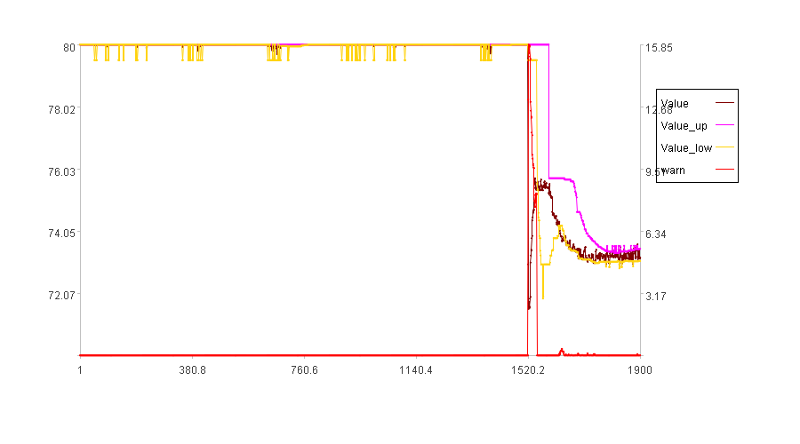
As the figure illustrates, the data within the channel is now considered normal, consistent with our intuitive assessment.
SPL Official Website 👉 https://www.esproc.com
SPL Feedback and Help 👉 https://www.reddit.com/r/esProcSPL
SPL Learning Material 👉 https://c.esproc.com
SPL Source Code and Package 👉 https://github.com/SPLWare/esProc
Discord 👉 https://discord.gg/sxd59A8F2W
Youtube 👉 https://www.youtube.com/@esProc_SPL

