A time series is a sequence of numerical values for a certain observed metric, arranged in chronological order. Examples in industrial settings include voltage readings from an electricity meter measured every second, hourly fuel flow rates, and daily production output of a product; these are all time series.

In statistical research, a time series is often represented by a set of variables arranged in chronological order, denoted concisely as X_t.

X_t=[x_t(0), x_t(1),…, x_t(n)]

where t(i) represents the i-th time point, x_t(i) is the value at the i-th time point, and n is the length of the time series X_t.

The time points in a time series are usually equally spaced, meaning that the sequence [t(i),…] is an arithmetic progression. This trivial sequence requires no special attention; we commonly use the number sequence as a substitute of the sequence t(i). From now on, unless otherwise stated, the time series X_t will be denoted as:

X= [x₁,x₂,…,x_n]

where x_i is the value at the i-th time point.

A segment of data before or after a specific time point in X is called interval data, or simply referred to as an interval. An interval is a contiguous subset of the time series X, and is also a time series.

The data in the interval of length k before x_i is denoted as X[-k]_i :

X[-k]_i=[x_i-k, x_i-k+2,…, x_i-2,x_i-1]

The data in the interval of length k after x_i is denoted as X[+k]_i:

X[+k]_i=[x_i+1, x_i+2,…, x_i+k-1,x_i+k]

The data at x_i combined with the data in the interval of length k before x_i are denoted as X[-(k+1)]_i+1.

Detecting anomalies in time series can be understood as a data mining task, that is, treat anomaly status as the target variable. However, data mining methods are a type of supervised learning, which requires prior labeling of which values are anomalies. Given that time series data is usually large and changes over time, accurate and timely labeling of massive historical data is impractical. Therefore, supervised learning cannot be used, making unsupervised learning the only feasible approach.

Then, in an unsupervised setting, i.e., without the need for labeling, how should “anomaly” be defined?

Simply put, we can assume that most data are normal (otherwise industrial production could not function properly), with only a small fraction being anomalous. Anomalies can be defined as data that have not occurred or occur infrequently. Therefore, anomaly detection becomes the task of identifying which data occur infrequently.

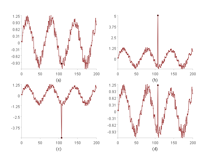
The figure above illustrates different scenarios for the same data at the same position (bold point). (a) represents normal data. (b) is anomalous due to its excessively large value. (c) is anomalous due to its excessively small value. (d) is a special, anomalous case distinct from the others. In summary, (b), (c), and (d) represent infrequent data points, and the goal is to identify them.

Determining if a data point is infrequent is to check if the current data x_i is infrequent compared to the previous interval data X[-k]_i. A pattern for determining if x_i is infrequent can be learned from X[-k]_i.

This pattern can be represented by a function, E(x), where the return value of E(x_i) determines if x_i is infrequent, i.e., is anomalous. Therefore, anomaly detection can be defined as the task of learning an anomaly function, E, from the historical data X[-k]_i, where E returns a boolean value (True/False or 0/1).

Clearly, even if we could write out functions in calculable forms, there would be too many forms, making it unlikely to try all functions. A practical approach is to first determine some commonly used function forms and leave their parameters undetermined. Therefore, the task of learning an anomaly function from X[-k]_i is, in fact, just determining the parameters.

More rigorously, first select a family of functions with a specific form and undetermined parameters.

E[a₁,…](x)=f(a_i,…,x)

where f is an expression with a definite form. Then, by learning from the historical data X[-k]_i, the parameters a1…, are determined, thereby specifying the function.

For example, consider the following function:

TA[tu,td](x)=if(max(x-tu, td-x,0)>0,1,0)

where tu and td represent the upper and lower threshold values, respectively, derived from learning X[-k]_i. The interval [td,tu] encompasses the majority of typical data points, while values outside this interval are considered infrequent anomalies. Thus, the function TA[tu,td] returns 1 to indicate an anomaly and 0 to indicate normal data. It can identify the anomalies illustrated in (b) and (c) of the figure above. The function family TA[tu,td] has two parameters, tu and td, which are to be determined. Once tu and td are determined by learning from X[-k]_i, the function is specified.

TA[tu,td] can be called a threshold-mode anomaly function. We will explore additional modes of anomaly functions in subsequent sections.

Experience indicates that in actual production processes, abnormal states often evolve gradually rather than abruptly. In this case, describing whether something is an anomaly simply using a boolean (True/False) value becomes somewhat simplistic, whereas employing a continuous value to measure the degree of abnormality provides richer information.

Thus, we revise the anomaly function E to return an anomaly score, i.e., the degree of abnormality. This is a real number, where a larger value corresponds to a greater anomaly score, and values exceeding 0 indicate an anomaly, while 0 indicates normal data.

For example, a slight modification of the threshold-based anomaly function mentioned earlier can yield a function that returns an anomaly score.

TA[tu,td](x)=max(x-tu, td-x,0)/(tu-td)

where tu and td retain their original meanings, and are still obtained by learning from the historical data X[-k]_i.

Based on our principle for anomaly detection, common data is considered normal, while infrequent data is considered anomalous. When setting k, the goal is to ensure that X[-k]_i contains mostly normal data, with few or no anomalies, at each time point. This implies that k should be larger when anomalies are expected to persist for longer periods, and smaller when anomalies persist for shorter periods. The appropriate k value should be set according to the actual situation.

In addition, if we learn from only the interval data X[-k]_i preceding the current time point, the limits of tu and td will be the maximum and minimum values of that interval, respectively. In this case, if the current time point’s data x_i is greater than the maximum value or less than the minimum value of X[-k]_i,, it will certainly be considered an anomaly. This assessment is often adequate in many production environments. However, in some production environments, it can still be considered normal when x_i is slightly larger or smaller than the previous data. Satisfying this requirement is simple: let x_i participate in the calculation of tu and td, that is, calculate tu and td using X[-(k+1)]i+1. As a result, if x_i is not extremely large or small, it is more likely that x_i becomes tu or td, and therefore be considered as normal.

Assuming the value at the current time point of a time series is x_i, and the sequence of the interval preceding it is X[-k]_i, the following sections present some commonly used detection methods to calculate the anomaly scores for x_i.