Associations between primary and sub tables, like orders and order details tables, are quite common. SQL uses JOIN to perform such associations, but performance often suffers significantly when both tables are large.

If both the primary and sub tables are pre-sorted by their primary keys, a merge algorithm can be used to perform association. This method requires only sequential traversal of the two tables, eliminating external storage buffering and drastically reducing I/O and computation.

esProc supports the ordered merge algorithm, which can greatly improve primary-subtable join performance. To illustrate this, we’ll compare the performance of esProc SPL and MySQL using an example involving orders and order details tables.

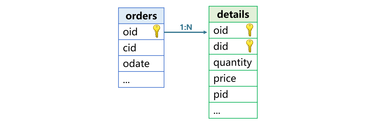
The MySQL database contains an orders table (10 million records) with primary key oid (order ID) and fields cid (customer ID) and odate (order date). The details table (30 million records) has a composite primary key of oid and did (detail ID), with fields quantity, price, and pid (product ID).

Test environment: VMware virtual machine with the following specifications: 8-core CPU, 8GB RAM, SSD. Operating system: Windows 11. MySQL version: 8.0.

First, download esProc at https://www.esproc.com/download-esproc/. The standard version is sufficient.

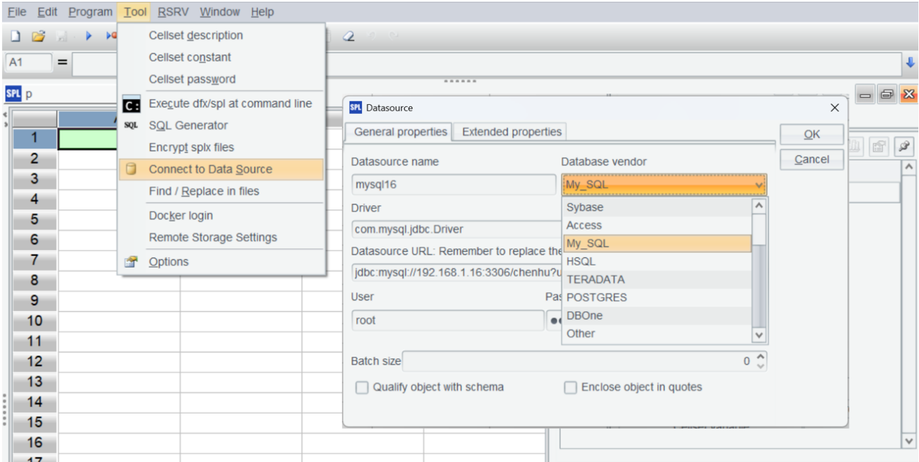
After installing esProc, test whether the IDE can access the database normally. First, place the JDBC driver of the MySQL database in the directory ‘[Installation Directory]\common\jdbc,’ which is one of esProc’s classpath directories.

Establish a MySQL data source in esProc:

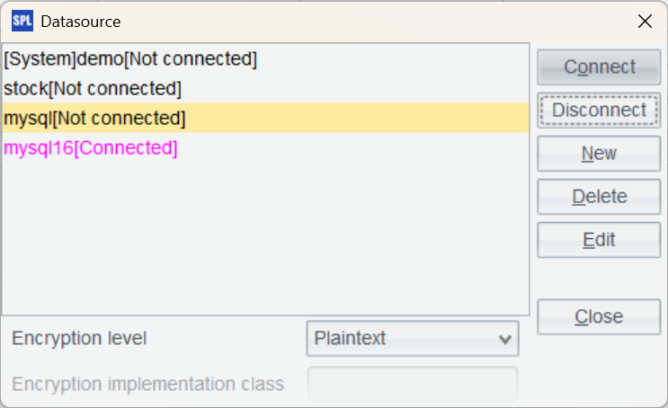
Return to the data source interface and connect to the data source we just configured. If the data source name turns pink, the configuration is successful.

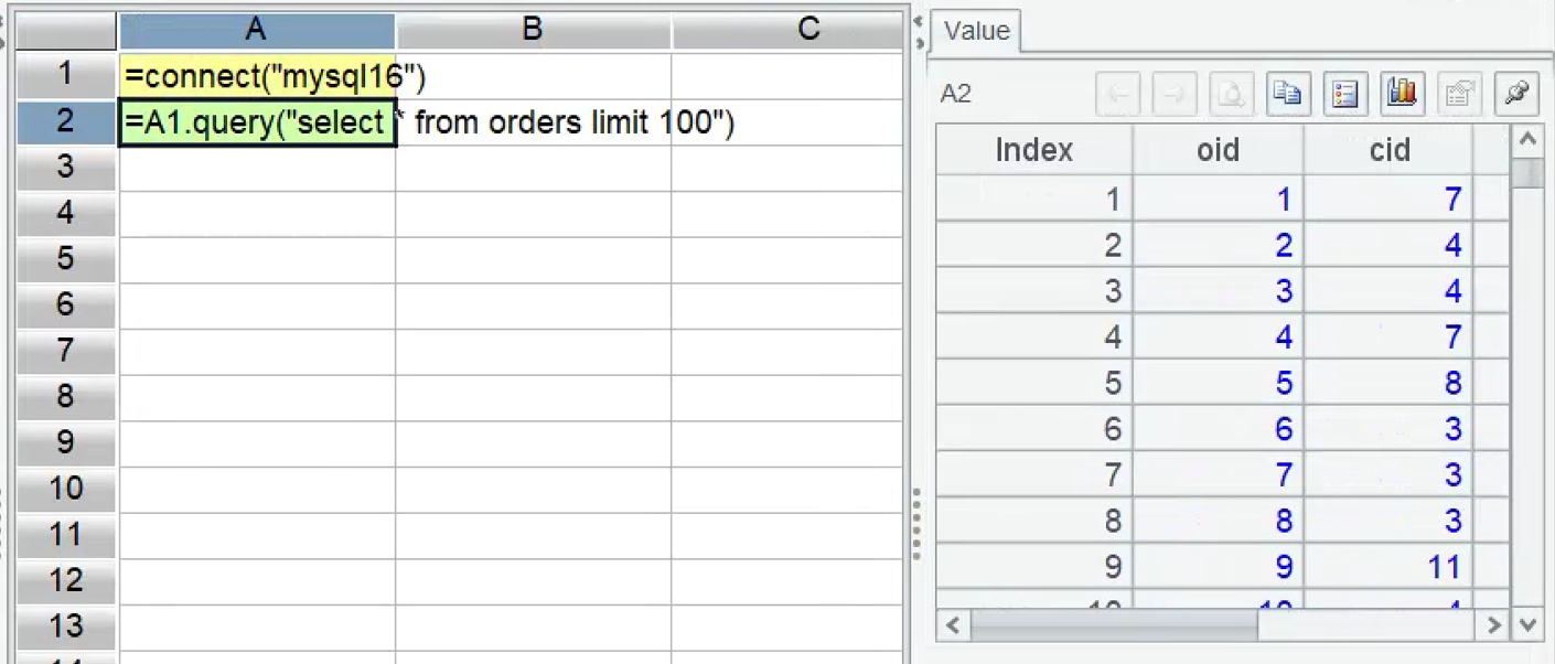
In the IDE, create a new script, write SPL statements to connect to the database, and execute a SQL query to load part of the data from the orders table.

	A	B
1	=connect("mysql16")
2	=A1.query("select * from orders limit 100")

Press Ctrl+F9 to execute the script. The result of A2 is displayed on the right side of the IDE, which is very convenient.

Next, prepare the data by exporting the historical data from the database to esProc’s high-performance files.

	A
1	=connect("mysql16")
2	=A1.cursor("select oid,cid,eid from orders order by oid")
3	=file("orders.ctx").create(#oid,cid,eid)
4	=A3.append(A1)
5	=A1.query("select oid,did,quantity,price from details order by oid")
6	=file("details.ctx").create@p(#oid,did,quantity,price)
7	=A6.append(A5)
8	>A1.close(),A3.close(),A6.close()

A2 generates a database cursor for the orders table.

A3 creates a composite table object, # indicating the composite table is ordered by oid. A4 appends data from the database cursor to the composite table.

A5 through A7 generate the details table in the same way. Note that the create function in A6 is affixed with the @p option because the association field oid in the subtable details is not unique. @p indicates the first field, oid, is a segmentation key, which prevents detail records for a single oid from being split during segmented reads.

With the data prepared, you can now use esProc to speed up primary-subtable joins.

Example 1: Calculate the total order amount, grouped by cid, within a specified date range.

select 
    o.cid,sum(d.quantity * d.price)
from 
    orders o
join 
details d on o.oid = d.oid
where o.odate>='2025-01-15'
	and o.odate<='2025-03-15'
group by o.cid;

MySQL failed to finish association on the two large tables after 10 minutes.

esProc uses ordered merge algorithm:

	A
1	=file("orders.ctx").open().cursor@m(oid,cid;odate>=date(2025,1,15) && odate<=date(2025,3,15))
2	=file("details.ctx").open().cursor(oid,quantity,price;;A1)
3	=joinx(A1:o,oid;A2:d,oid)
4	=A3.groups(o.cid;sum(d.quantity*d.price))

It’s important to note that the last parameter of the cursor in A2 is A1, indicating that for multi-threaded parallel processing, details will be segmented following orders to ensure the correctness of the subsequent ordered merge of the two tables.

A3 performs an ordered merge join of orders and details; A4 then groups and aggregates the results.

Execution time: 1.7 seconds.

Example 2: Calculate the total order amount, grouped by <pid, for orders with cid 3 or 9.

select 
    d.pid,sum(d.quantity * d.price)
from 
    orders o
join 
details d on o.oid = d.oid
where o.cid =3
	or o.cid=9
group by d.pid;

MySQL also failed to produce a result after 10 minutes.

esProc code:

	A
1	=file("orders.ctx").open().cursor@m(oid;cid==3 || cid==9)
2	=file("details.ctx").open().cursor(oid,quantity,price,pid;;A1)
3	=joinx(A1:o,oid;A2:d,oid)
4	=A3.groups(d.pid;sum(d.quantity*d.price))

Execution time: 1.8 seconds.

Example 3: Calculate the average amount per order, grouped by odate, for order details with pid not 2 or 8.

select o.odate,
sum(d.quantity * d.price)/count(distinct o.oid) 
from orders o 
    join details d on o.oid = d.oid 
where d.pid !=2 and d.pid !=8 
group by o.odate; 

MySQL still failed to produce a result after 10 minutes.

The code involves a primary-subtable join followed by a distinct count, both of which exhibit poor performance in SQL. esProc’s ordered distinct count offers significantly better performance. Moreover, since ordered distinct count also requires the data to be ordered by oid, it can be easily implemented after the ordered merge.

esProc code:

	A
1	=file("orders.ctx").open().cursor@m(oid,odate)
2	=file("details.ctx").open().cursor(oid,quantity,price;pid!=2 && pid!=8;A1)
3	=joinx(A1:o,oid;A2:d,oid)
4	=A3.groups(o.odate;sum(d.quantity*d.price)/icount@o(o.oid))

In A4, icount@o represents the ordered distinct count.

Execution time: 4 seconds.

esProc dramatically outperforms MySQL in associating between large primary and sub tables.

esProc’s speedup solution requires primary and sub tables to be stored in order by primary key oid. If there is new data, which is typically new oid values, you can append them directly to the existing composite table.

If historical data needs to be changed – for example, modified, inserted, or deleted – things become a little bit cumbersome. When the amount of changed data is small, it can be written to a separate supplementary area. During reading, the supplementary area and normal data are merged and computed together, resulting in a seamless experience.

When the amount of changed data is large, it needs to regenerate the full ordered data, but it is a time-consuming process and cannot be done frequently.

In practice, numerous computational scenarios rely on static historical data, and many joins between large primary and sub tables urgently need performance improvements. SPL ordered storage can effectively speed up these scenarios, and implementation is remarkably straightforward.