

SPL Quantitative Trading Practice Series: Linear Regression Strategy
In the stock market, there may be a linear relationship between the stock price on the current day and stock prices in several previous trading days. According to this concept, we design the following strategy:
1. Use data of the 100 trading days before the current day as the training data;
2. Among the training data, set closing price on each day’s next day as the target variable;
3. Among the training data, use the opening price, the highest price, the lowest price and the closing price of each day’s recent M days as the metrics;
4. Perform Principal Component Analysis (PCA) on those metrics and extract the first four principal components;
5. Perform linear regression using the principal components and the target variables in the training data to get a linear model;
6. Use the linear model to predict principal components of the data in the recent M days to get y_predict;
7. If y_predict>current day’s closing price, mark it as the buy signal (signal=1); otherwise mark it as the sell signal (signal=-1);
8. When signal=1 and no position is held, place an order to buy; and when signal=-1 and positions are held, place an order to sell. Generate the buy/sell signal (flag) according to the prediction result – make purchases when flag=1, perform selling when flag=-1, and take no action when flag=0.
In this example we set value of M as 5.
SPL code:
| A | |
|---|---|
| 1 | =file(“daily/300750.csv”).import@tc() |
| 2 | =A1.select(trade_date>20200101&&trade_date<=20231231) |
| 3 | =A2.derive(if(#>1, close/ pre_close *factor[-1], close/pre_close):factor) |
| 4 | =hfq_fst=A3(1),A3.derive((fcls=factor/hfq_fst.factor*hfq_fst.close,c=fcls/close,round(c*open,2)): hfq_open,round(c*high,2): hfq_high,round(c*low,2): hfq_low,round(fcls,2): hfq_close) |
| 5 | =M=5 |
| 6 | =trdata=100 |
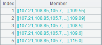
| 7 | =A4.([~[-M+1:0].conj([hfq_open,hfq_high,hfq_low,hfq_close]),~[1].hfq_close]) |
| 8 | =A4.pselect@a(trade_date>=20230101) |
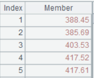
| 9 | =A7.calc(A8,(data=~[-trdata,-1],train=data.(~(1)),pc_res=pca(train,4),pc=pca(train,pc_res),target=data.(~(2)),model=linefit(pc.(~|1),target),pdata=[~(1)],pc_pdata=pca(pdata,pc_res),round(mul(pc_pdata.(~|1),model),2))) |
| 10 | =ps=0,A4(A8).derive(A9(#):predict,if(predict>hfq_close,1,-1):signal,if(ps==0&&signal==1,(ps=1,1),if(ps!=0&&signal==-1,(ps=0,-1),0)):flag,if(flag!=0,100,0):shares) |
A4: Backward adjust the stock price. The result includes “open”, “high”, “low” and “close” values.
A7: Concatenate metrics and compute target variable.
A9: Time rolling calculation. Perform data training, including PCA computation and linear regression analysis, using data of the previous 100 trading days, and then prediction using data of the previous days to obtain the predicted stock price in the next trading day.
Note: SPL designs the order-based computations meticulously. The calc()method in A9, for example, performs PCA analysis on each trading day’s data and builds a model to predict closing price of the next day after it gets index of stock prices in 2023. In the computation, [] is used to get neighboring data. The syntax gets rid of the complicated for loop and makes it convenient to express the algorithm. This is an ability that other languages, like Python, do not have.
A10: Determine the signal to buy or sell (signal) using the predicted stock price, compute buy/sell signal flag (flag), and specify the order quantity (100 shares).

Plot a buy/sell signal chart according to A10’s data:
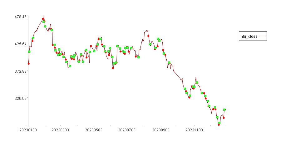
In the above chart, red dots represent buy points and green squares are sell points.
Same as what is explained in SPL Quantitative Trading Practice Series: Turtle Trading Strategy, compute the flag and then we can do the backtesting. Just get records where flag values are not 0 from A10’s result set and call the backtesting interface.
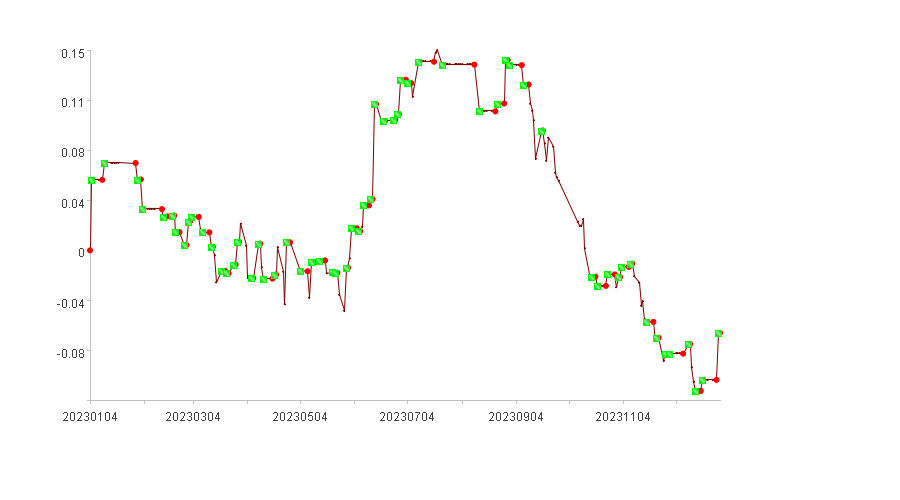
The following chart displays the backtested RoRs:
The following table lists backtested indicators:
| Indicators | Value |
|---|---|
| Cumulative rate of return | -6.24% |
| Annualized rate of return | -6.52% |
| Annual volatility | 18.4% |
| Sharpe ratio | -0.52 |
| Maximum drawdown | 22.35% |
| Cash invested | 44255.45 |
| Total assets | 41493.28 |
| Stock holding ratio | 71.29% |
| Profits count | 29 |
| Losses count | 30 |
SPL Official Website 👉 https://www.esproc.com
SPL Feedback and Help 👉 https://www.reddit.com/r/esProcSPL
SPL Learning Material 👉 https://c.esproc.com
SPL Source Code and Package 👉 https://github.com/SPLWare/esProc
Discord 👉 https://discord.gg/sxd59A8F2W
Youtube 👉 https://www.youtube.com/@esProc_SPL


Chinese version