The MACD (Moving Average Convergence Divergence), derived from the Exponential Moving Average (EMA), is highly effective for capturing trending market conditions. Its top (bearish) and bottom (bullish) divergences serve as a proven method for “buying the dip and selling the peak”, making it a key consideration for many medium- to long-term investors in real-world trading. In this essay, we will implement the MACD divergence strategy using SPL (Structured Process Language) and conduct backtesting to evaluate its performance.

Before offering the SPL code, we need to look at how to compute MACD:

1. Short-term EMA: The short-term exponential moving average. The moving timeframe for it is typically 12 days.

EMA=q*closing price+(1-q)* EMA[-1]

In the formula, q is the smoothing coefficient, whose value is q=2/(moving timeframe +1), and closing price is the backward adjusted price.

All subsequent EMAs will be computed in this way, only with different moving timeframes.

2. Long-term EMA: The long-term exponential moving average. The moving timeframe for it is typically 26 days.

3. Deviation between short-term EMA and long-term EMA (DIFF): short-term EMA - long-term EMA.

4. Double Exponential Moving Average (DEA): The DIFF’s exponential moving average. The moving timeframe for it is typically 9 days.

5. MACD：2 *(DIFF - DEA)

Then move on to learn about the MACD trading strategy:

Golden Cross: It occurs when DIFF crosses above the DEA.

Death Cross: It occurs when DIFF crosses below the DEA.

Bullish divergence: When the stock price hits a new low but the DIFF does not reach a new low, define the period from the most recent death cross to the golden cross as Interval 1, and the preceding death cross to golden cross period as Interval 2. If the lowest stock price in Interval 1 is lower than that in Interval 2, while the lowest DIFF value in Interval 1 is higher than that in Interval 2, the golden cross at this point serves as a buy signal.

Bearish divergence: When the stock price hits a new high but the DIFF does not reach a new high, define the period from the most recent golden cross to the death cross as Interval 3, and the preceding golden cross to death cross period as Interval 4. If the highest stock price in Interval 3 is higher than that in Interval 4, while the highest DIFF value in Interval 3 is lower than that in Interval 4, the death cross at this point serves as a sell signal.

SPL code:

	A
1	=file(“daily/000026.csv”).import@tc()
2	=A1.select(trade_date>=20200101&&trade_date<=20240306)
3	=A2.derive(if(#>1, close/ pre_close *factor[-1], close/pre_close):factor)
4	=hfq_fst=A3(1),A3.derive(round(factor/hfq_fst.factor*hfq_fst.close,2): hfq_close)
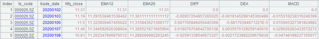
5	=q12=2/13,q26=2/27,q9=2/10,A4.new(ts_code,trade_date,hfq_close,if(#==1,hfq_close,q12*hfq_close+(1-q12)*EMA12[-1]):EMA12,if(#==1,hfq_close,q26*hfq_close+(1-q26)*EMA26[-1]):EMA26,EMA12-EMA26:DIFF,if(#==1,DIFF,q9*DIFF+(1-q12)*DEA[-1]):DEA,2*(DIFF-DEA):MACD)
6	=lth=A5.len(),A5.derive(if(#==1,0,if(DIFF>DEA&&DIFF[-1]<DEA[-1],1,if(DIFF<DEA&&DIFF[-1]>DEA[-1],-1,0))):gcross_or_dcross,0:signal)
7	=A6.pselect@a(gcross_or_dcross!=0)
8	=A7.(if(#==1,,to(~[-1],~))).to(2,)
9	=A8.group((#-1)%2)
10	=s=A6(A7(1)).gcross_or_dcross,if(s==1,A9.rvs(),A9)
11	=A10(1).(A6(~)).((itv1=~,itv2=~[-1],if(#>1&&itv1.min(hfq_close)<itv2.min(hfq_close)&&itv1.min(DIFF)>itv2.min(DIFF),~.m(-1).signal=1)))
12	=A10(2).(A6(~)).((itv1=~,itv2=~[-1],if(#>1&&itv1.max(hfq_close)>itv2.max(hfq_close)&&itv1.max(DIFF)<itv2.max(DIFF),~.m(-1).signal=-1)))
13	=ps=0,A6.derive(if(ps==0&&signal==1,(ps=1,1),if(ps!=0&&signal==-1,(ps=0,-1),0)):flag,if(flag!=0,100,0):shares)

A4: Backward adjust the closing price.

A5: Compute MACD indicators, including EMA, DIFF, DEA and bars in MACD.

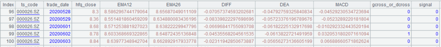
A6: Compute golden cross and death cross – the golden cross occurs when gcross_or_dcross=1, the death cross occurs when gcross_or_dcross=-1, and in all other time gcross_or_dcross=0, and add a buy/sell signal field (signal) whose initial value is set as 0.

A7: Get positions of the golden cross or death cross.

A8: Divide records into intervals from golden cross to death cross and from death cross to golden cross.

A9: If the interval from golden cross to death cross is at odd-numbered positions, then that from death cross to golden cross is at the even-numbered position, and vice versa.

A10: If members of the first group are intervals from golden cross to death cross, reverse the order of the two groups to make sure they are intervals from death cross to golden cross; if they are not, keep the existing order.

A11: Generate buy/sell signals based on bullish divergence rules. If a bullish divergence occurs, set signal=1 at the corresponding golden cross position.

A12: Determine bearish divergence signal in the same way and represent it with signal=-1. Here are records with adjusted signals:

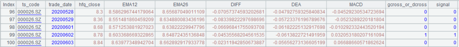
Previously in A6, we add a signal field and make 0 its initial values. A11 and A12 then use index to get A6’s records and modify signal values after a series of operations. This is thanks to SPL support of discrete data, which allows records to be independent of the table sequence. The modification of discrete records is also synced to the original records. It is natural and simple, and we can write code in this way. With Python, DataFrame is usually copied. Modifying the copied DataFrame won’t result in the update of the original data. To modify the original data, we can only first obtain their indexes and change target field values directly on them. Yet this approach leads to roundabout code.

A13: If no position is held and a buy signal appears, buy 100 shares; otherwise, take no action. If a position is held and a sell signal appears, sell 100 shares; otherwise, take no action.

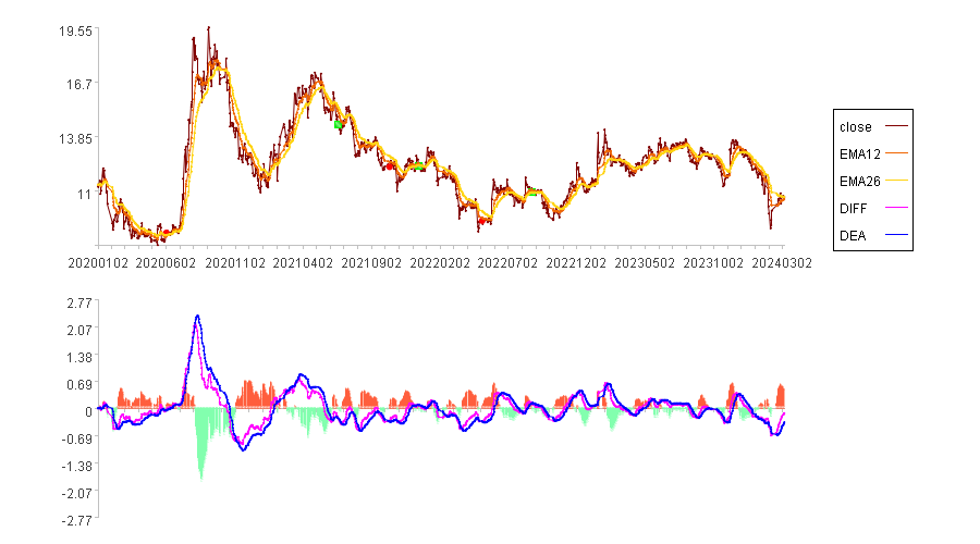
Plot the MACD histogram according to the above result data (Only part of the chart is displayed here for clear viewing):

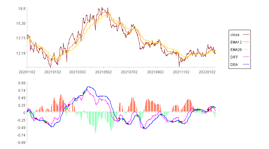
In the above chart, the upper part displays stock prices and short-term and long-term EMAs; the lower part shows MACD’s DIFF, DEA and red and green bars of MACD. The red dots represent golden crosses and green squares are death crosses.

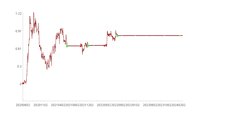
We can also plot a buy/sell chart according to the same data:

In the above chart, red dots are buy points, and green squares are sell points.

Same as what is explained in SPL Quantitative Trading Practice Series: Turtle Trading Strategy, compute the flag and then we can do the backtesting. Just get records where flag values are not 0 and call the backtesting interface.

Below is the chart displaying backtested RoRs:

The following table lists backtested indicators:

Indicators	Value
Cumulative rate of return	82.22%
Annualized rate of return	17.23%
Annual volatility	50.06%
Sharpe ratio	0.28
Maximum drawdown	44.18%
Cash invested	883.01
Total assets	1609.01
Stock holding ratio	0.0%
Profits count	3
Losses count	0