SQL’s JOIN definition is very simple. It is the filtered Cartesian product of two tables, represented by syntax A JOIN B ON …. The general definition does not capture the essence of JOIN operations, creating difficulties in coding and optimization.

SPL redefines joins by disconnecting them from the Cartesian product and dividing them into two types – foreign key-based joins and primary key-based joins.

SPL uses different functions to deal with different types of joins, which reflects JOIN operation’s nature. This allows users to use different methods even different storage strategies according to characteristics of different joins so that computations will become faster.

One type of joins is foreign key-based join, where a table’s ordinary field (foreign key) is associated with the other table’s primary key. Both the relationship between orders table and customer table and that between orders table and shipper table are foreign-key based.

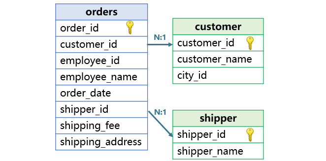
A table’s foreign key is the related table’s primary key, whose values are unique. SPL regards the foreign key as an object.

Note that the primary key mentioned above is a logical one, whose values are unique in the table. The field isn’t necessarily the primary key set on the physical table, and neither is a foreign key.

The other type of joins is primary key-based. A primary key-based join creates association between a table’s primary key and another table’s primary key or part of a composite key. For example, orders table’s primary key (order_id) is associated with the corresponding field of the primary key in details table.

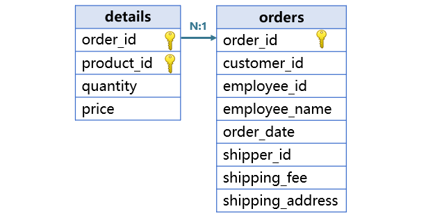
SPL treats the primary key-based join as an association between record objects or sets of records.

It is necessary to point out that the foremost part of using SPL to handle joins is to correctly determine the join type. Only after you know which type of joins you are dealing with, you can choose the suitable method. The key to a correct determination is to examine the primary key’s role in the join.

Take the following tables (orders, customer, city, state and shipper) as examples, let’s look at how esProc SPL speeds up foreign key-based joins through external data querying.

Define a Q3.etl using the ETL tool. Drag in tables involved in the computation:

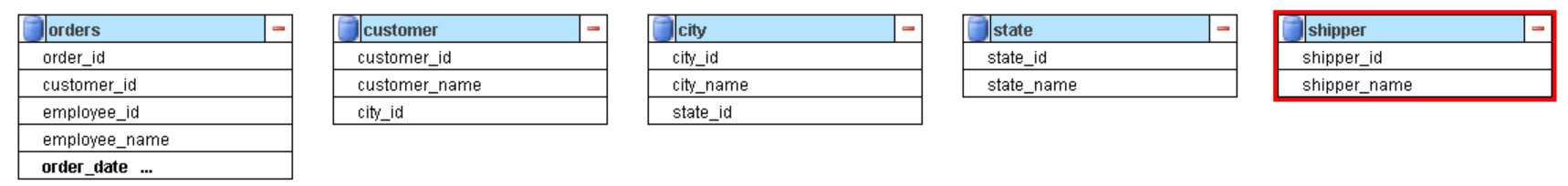
orders is the fact table, which is the largest. For the convenience of coding, dump it into a CTX file, and each of the smaller dimension tables in a BTX file.

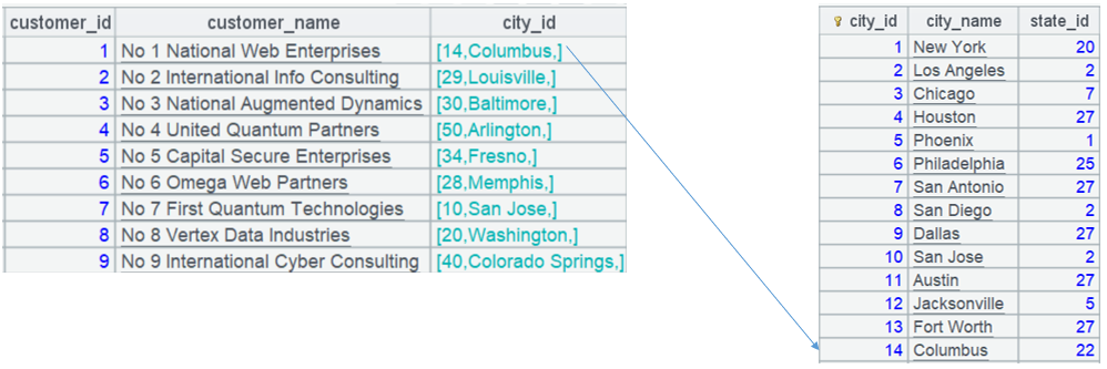
Perform the following settings to numberize the related field. For example, convert values of customer table’s city_id field to index values in dimension table city.

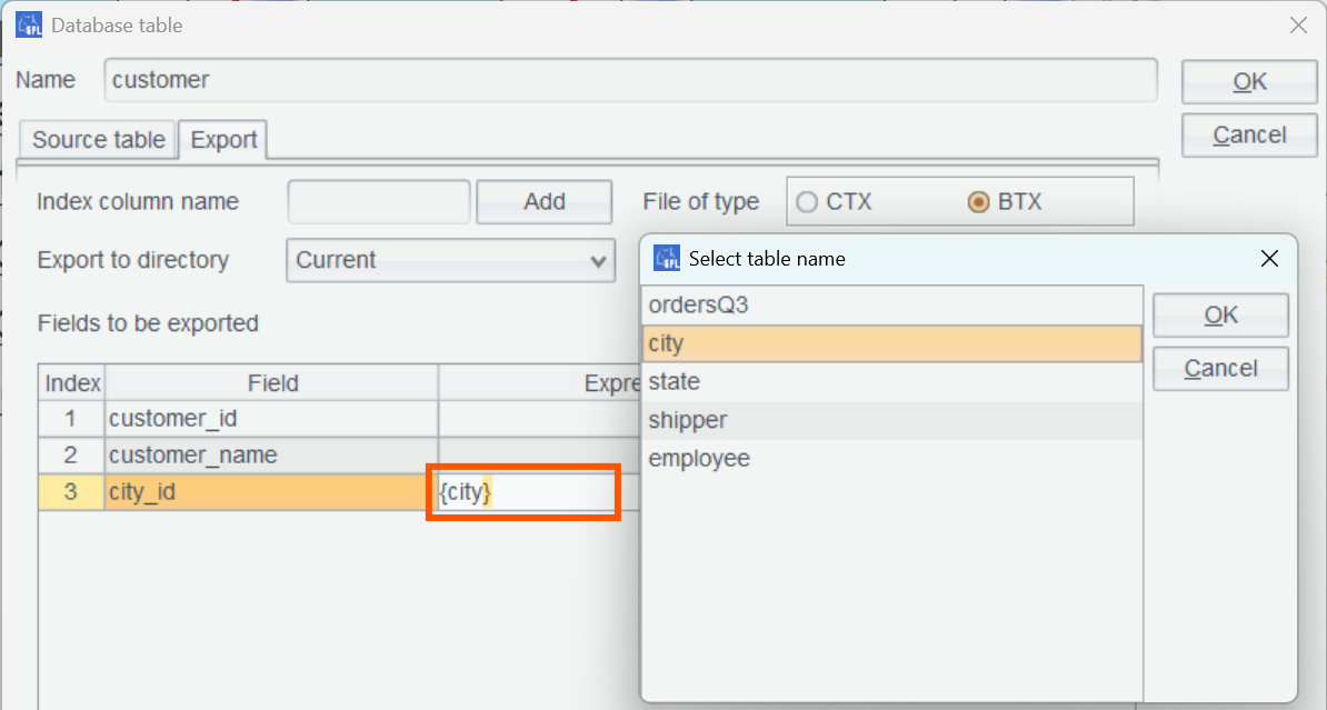
Double-click the blank space at “Expression/Numberized Table” and select city table. Similarly, create a state table based on city table’s state_id field.

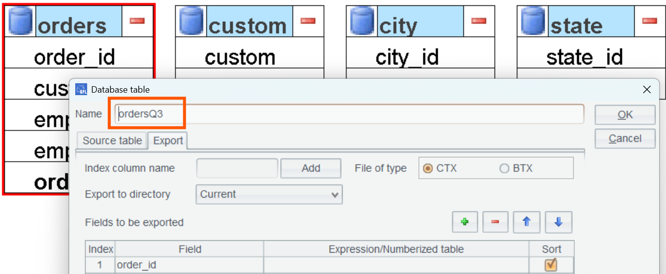
Change name of orders table to ordersQ3 (to differentiate it from the previous one):

employee_name does not have a corresponding dimension table, so all its values need to be obtained from table orersQ3. Create dimension table employee:

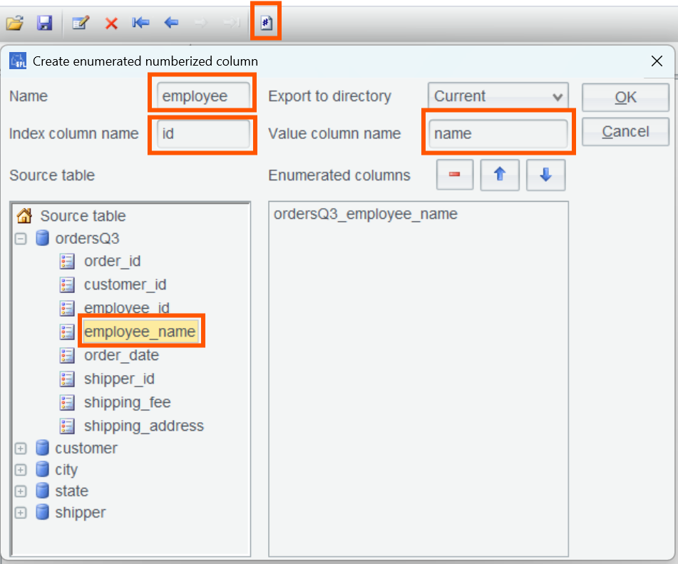
The order of operations in the above window: 1. Click Create Enumerated Numberized Column; 2. Double-click employee_name; 3. Define dimension name employee; 4. Define dimension table’s Index Column Name as id; 5. Define dimension table’s Value Column Name as name.

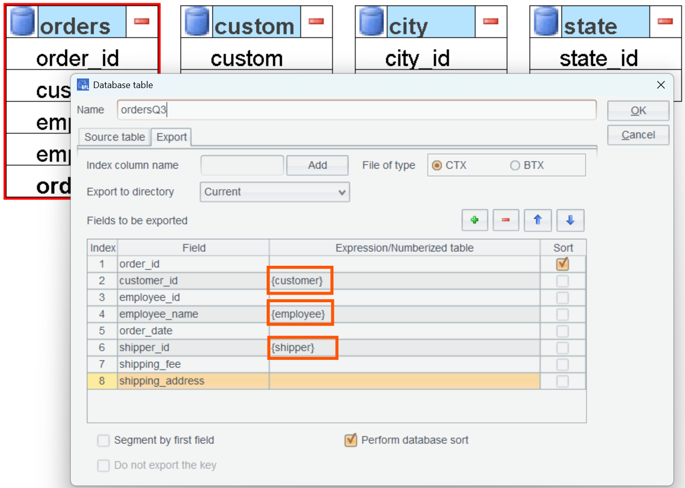
Then set the numberized field in ordersQ3:

SPL code example 14: Export data and dump them to BTX or CTX files.

	A
1	=connect("speed")
2	="d:\\speed\\etl\\"
3	=A1.query("SELECT Distinct employee_name FROM orders")
4	=A3.(employee_name).new(#:id,~:name).keys@i(name)
5	=file(A2+"employee.btx").export@b(A4)
6	=A1.query("SELECT state_id,state_name FROM state ORDER BY state_id")
7	=A6.keys@i(state_id)
8	=file(A2+"state.btx").export@b(A6)
9	=A1.query("SELECT city_id,city_name,state_id FROM city ORDER BY city_id")
10	=A9.new(city_id,city_name,A7.pfind(state_id):state_id).keys@i(city_id)
11	=file(A2+"city.btx").export@b(A9)
12	=A1.query("SELECT customer_id,customer_name,city_id FROM customer ORDER BY customer_id")
13	=A12.new(customer_id,customer_name,A10.pfind(city_id):city_id).keys@i(customer_id)
14	=file(A2+"customer.btx").export@b(A12)
15	=A1.query("SELECT shipper_id,shipper_name FROM shipper ORDER BY shipper_id")
16	=A15.keys@i(shipper_id)
17	=file(A2+"shipper.btx").export@b(A15)
18	=A1.cursor("SELECT order_id,customer_id,employee_id,employee_name,order_date,shipper_id,shipping_fee,shipping_address FROM orders ORDER BY order_id")
19	=A18.new(order_id,A13.pfind(customer_id):customer_id,employee_id,A4.pfind(employee_name):employee_name,order_date,A16.pfind(shipper_id):shipper_id,shipping_fee,shipping_address)
20	=file(A2+"ordersQ3.ctx").create@y(#order_id,customer_id,employee_id,employee_name,order_date,shipper_id,shipping_fee,shipping_address).append(A19).close()
21	=A1.close()

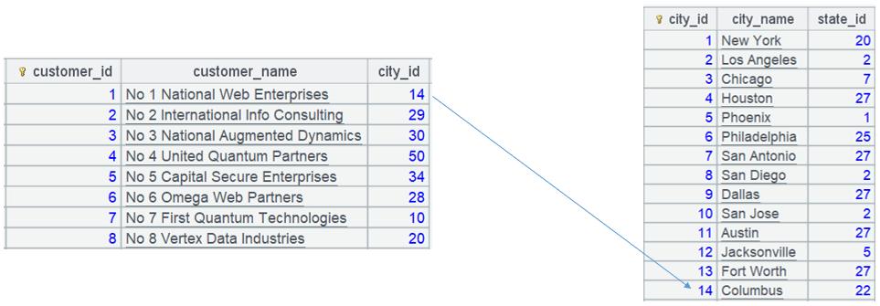
In A13, pfind() function converts valus of customer table’s city_id field to corresponding dimension table city’s indexes:

SPL code example 15: Perform initialization at the system startup or data update.

	A	B
1	=file("state.btx").import@b()	=env(state,A1)
2	=file("city.btx").import@b()	=env(city,A2)
3	=file("customer.btx").import@b()	=env(customer,A3)
4	=file("shipper.btx").import@b()	=env(shipper,A4)
5	=city.run(state_id=state(state_id))
6	=customer.run(city_id=city(city_id))

Perform initialization to preload each of the dimension tables into the memory and use env() function to store it as a global variable.

Perform pre-association by using run() function to convert foreign key values to the corresponding records in the dimension table, as A6 does:

Values of the regular field city_id in table sequence customer are transformed to corresponding city table records.

After data is dumped and initialized, actual computations begin. Here is an example:

Example 3.1 Group orders from a specified state by shipper and compute freights in each group (include shipper name in the result).

SQL statement:

select shipper.shipper_id, shipper.shipper_name,sum(o.shipping_fee)
from 
    orders o
join 
    customer c on o.customer_id = c.customer_id
join 
    city on city.city_id = c.city_id
join 
    state on state.state_id = city.state_id
join 
    shipper on o.shipper_id = shipper.shipper_id
where 
    state.state_name = 'California'
group by 
 shipper.shipper_id, shipper.shipper_name;

It takes 20 seconds to finish executing the above SQL code.

SPL code example 16:

	A
1	=now()
2	=file("ordersQ3.ctx").open()
3	=A2.cursor@m(order_id, customer_id,shipper_id,shipping_fee;customer_id:customer:#,shipper_id:shipper:#)
4	=A3.select(customer_id.city_id.state_id.state_name=="California").groups(shipper_id;shipper_id.shipper_name,sum(shipping_fee))
5	>output("query cost:"/interval@ms(A1,now())/"ms")

In A3, syntax customer_id:customer:# creates association between orders records and customer table on the cursor according to sequence number #. Once the join operation is finished, values of both customer_id and shipper_id will be converted to record objects in the corresponding tables.

As associations between dimension tables are already created at the initialization, A3 can use object properties to write the code: customer_id.city_id.state_id.state_name.

It takes 0.4 second to finish executing the SPL script.

Example 3.2 Group records by cities where customers are based and find the number of orders in each group (include state name and city name in the result).

select city.city_id,city.city_name,state.state_name,count(o.order_id)
from 
    orders o
join 
    customer c on o.customer_id = c.customer_id
join 
    city  on c.city_id = city.city_id
join 
    state on city.state_id = state.state_id
group by 
city.city_id,city.city_name,state.state_name;

It takes 22 seconds to finish executing the SQL code.

SPL code example 17: Based on the preceding SPL code example 16, just change A4’s code:

	A
1	=now()
2	=file("ordersQ3.ctx").open()
3	=A2.cursor@m(order_id, customer_id,shipper_id,shipping_fee;customer_id:customer:#,shipper_id:shipper:#)
4	=A3.groups(customer_id.city_id.city_id;customer_id.city_id.city_name,customer_id.city_id.state_id.state_name, count(1))
5	>output("query cost:"/interval@ms(A1,now())/"ms")

It takes 0.3 second to finish executing the SPL code.

Performance summary (unit:second):

	MYSQL	SPL
Example 3.1	20	0.4
Example 3.2	22	0.3

Exercises:

1. Find order records where the shipper names are Elite Shipping Co., group them by states where customers are based, and compute freight in each group (include state in the result).

2. Critical thinking: Do you have any tables related via foreign keys in one of your familiar databases? Can you use the numberization method to speed up joins between them?