Mixed computations between different structure data coming from multiple sources are more commonly seen. One example is the analysis involving different business systems.

Data structure description

The vehicle management system (DB_Vehicle) stores information related to vehicles and owners. Here is a simple description of the structure of owner information table (owner_info):

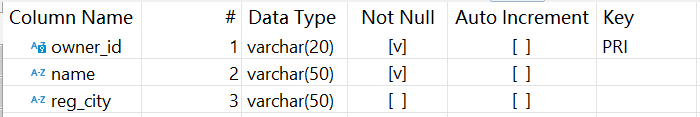
The primary key owner_id stores the owner IDs.

Below is a simple description of the structure of vehicle table (vehicle_master):

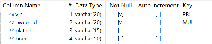
vin field is the primary key and plate_no values are unique. Both fields can be logically treated as primary keys.

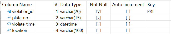
Traffic Management System (DB_Traffic) stores vehicle traffic information. Below is the structure of traffic violation table (traffic_violation):

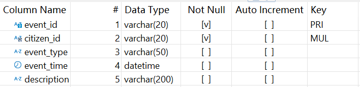
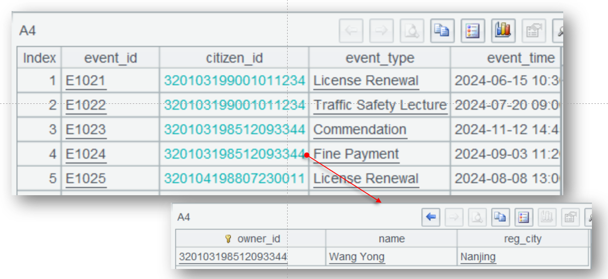
Citizen Information System (DB_CitizenEvent) stores information related to citizens. Below is structure of citizen events table (citizen_event):

Below shows logical relations between the four tables:

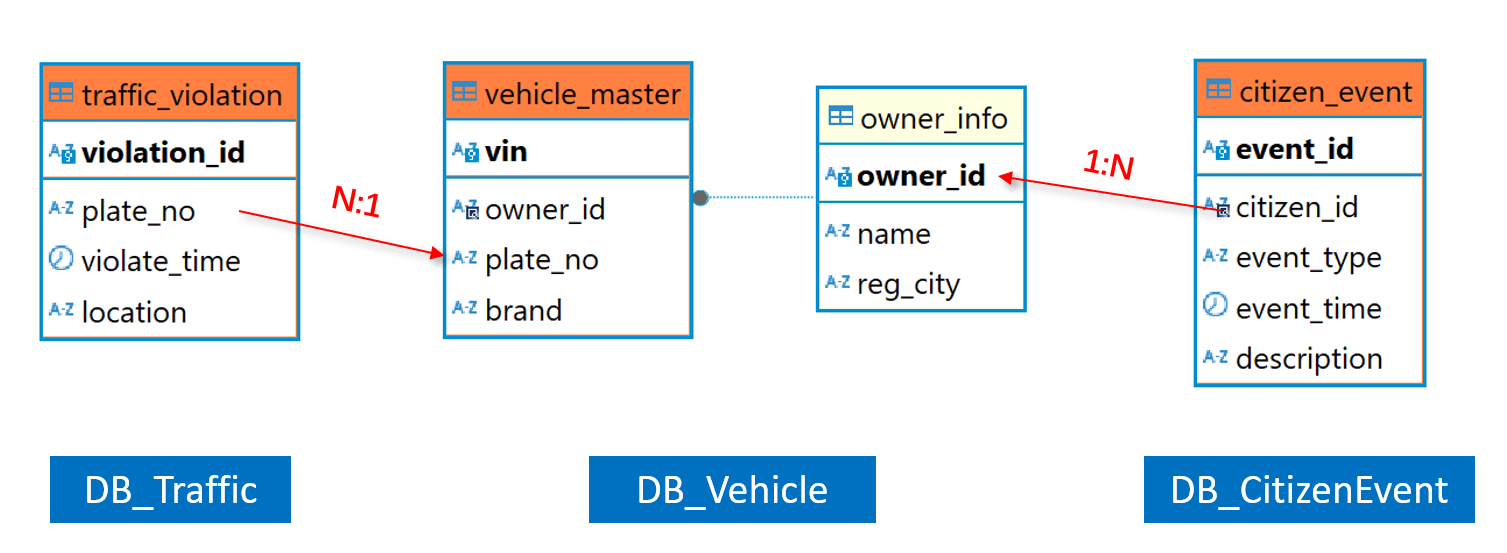
Logically, there is a one-to-many relation between owner_info and citizen_event. The latter, as the dimension table, is much smaller than the former.

vehicle_master and traffic_violation also have a one-to-many relationship, and probably both are large. Seeing from vehicle_master table, traffic_violation table is more like the subtable. The two tables form a primary-sub table relationship (plato_no is vehicle_master table’s logical primary key).

Why is it important to distinguish different types of relationships between tables?

Basically, most equi-joins involve the primary key (many-to-many relationship nearly does not have any business significance). Generally, there are two types of equi-joins. One is dimension-based join, which happens between a table’s ordinary field and the dimension table’s primary key (like the one between citizen_event and owner_info). The other is the join between a table’s primary key and another table’s primary key or part of its primary keys (like the one between vehicle_master and traffic_violation /traffic_violation; in traffic_violation, plate_no and violation_id forms a compound key, where the latter is in the subordinate position).

SPL can choose the most suitable method to deal with a JOIN computation according to the JOIN type, simplifying code and increasing efficiency.

Setting up data source connection

vehicle：

jdbc:mysql://127.0.0.1:3306/db_vehicle?useSSL=false&useCursorFetch=true

traffic：

jdbc:mysql://127.0.0.1:3306/db_traffic?useSSL=false&useCursorFetch=true

citizen:

jdbc:mysql://127.0.0.1:3306/db_citizenevent?useSSL=false&useCursorFetch=true

Computing use case

We have the following computing goals:

1. Count the number of personal vehicle events in the past year in each city to analyze the activity level of this city’s vehicle owners.

2. Find names of vehicle owners who get commended and descriptions of their events in order to identify Outstanding Citizens.

3. Count the frequency of traffic violations for each car brand in each year in order to find whether certain brands of cars are more likely to violate traffic rules. The result will be used for studying the correlation between driving behavior and car brands.

Let’s look at the first computing goal: Count the number of personal vehicle events happened to car owners in the past year in each city. This involves the join between owner_info and citizen_event, which is a dimension-based join.

Dimension-based join

esProc implementation:

	A
1	=connect("vehicle")
2	=A1.query@x("select * from owner_info").keys@i(owner_id)
3	=connect("citizen")
4	=A3.query@x("select * from citizen_event where event_time >= DATE_SUB(CURDATE(), INTERVAL 1 YEAR)")
5	=A4.switch(citizen_id,A2)
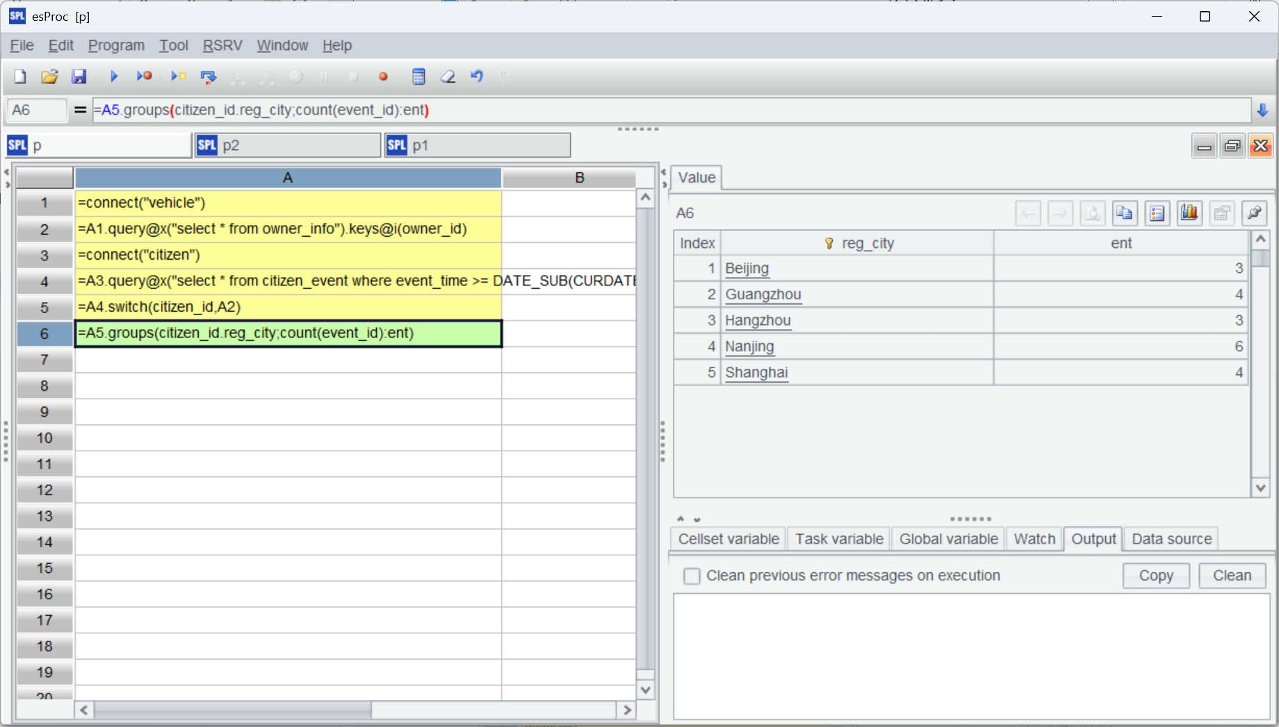
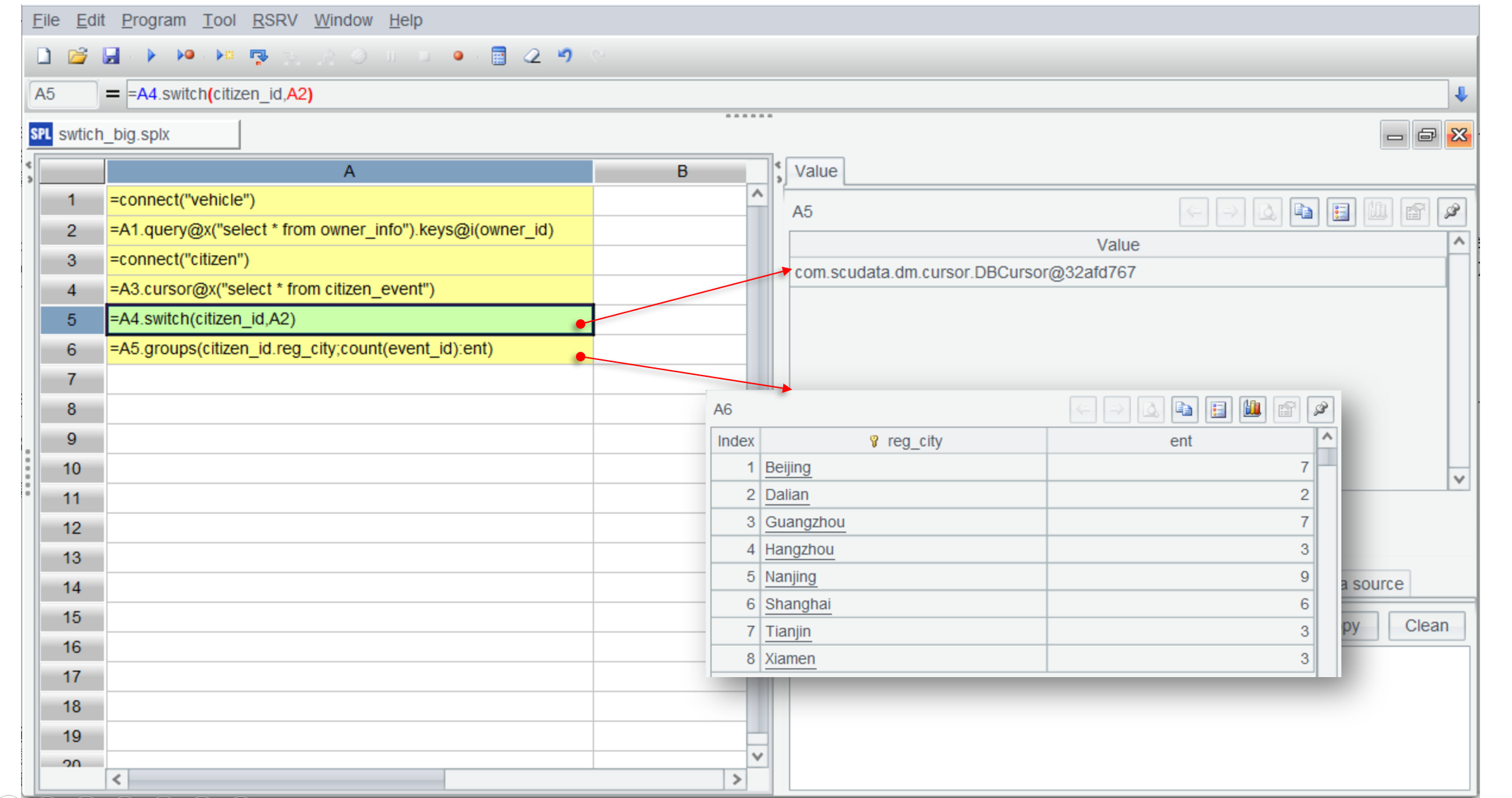
6	=A5.groups(citizen_id.reg_city;count(event_id):ent)

A2 queries owner information from vehicle database. query@x means closing the database connection after all data is loaded to the memory; and keys@i sets up primary key and creates an index. The fact table is usually much larger than the dimension table, and the index will be repeatedly reused to speed up the computation.

A4 queries citizen_event table to read records of the past year into the memory.

A5 uses switch()function to perform foreign key-based join. Since the dimension table record pointed by the foreign key is unique, the function directly converts the associated field citizen_id to the corresponding record in A2 (actually it is the address of dimension record that is stored in the memory).

The conversion is once for all. Its result can be repeatedly used by the subsequent computations. It can handle foreign key-based associations with multiple dimension tables at a time. After the association is created, we can use the “associated field.dimension table field” syntax to reference any field of the dimension table. Using this method, A6 gets registration city through citizen_id.reg_city to perform grouping and aggregation.

Execute the script and we get the final result:

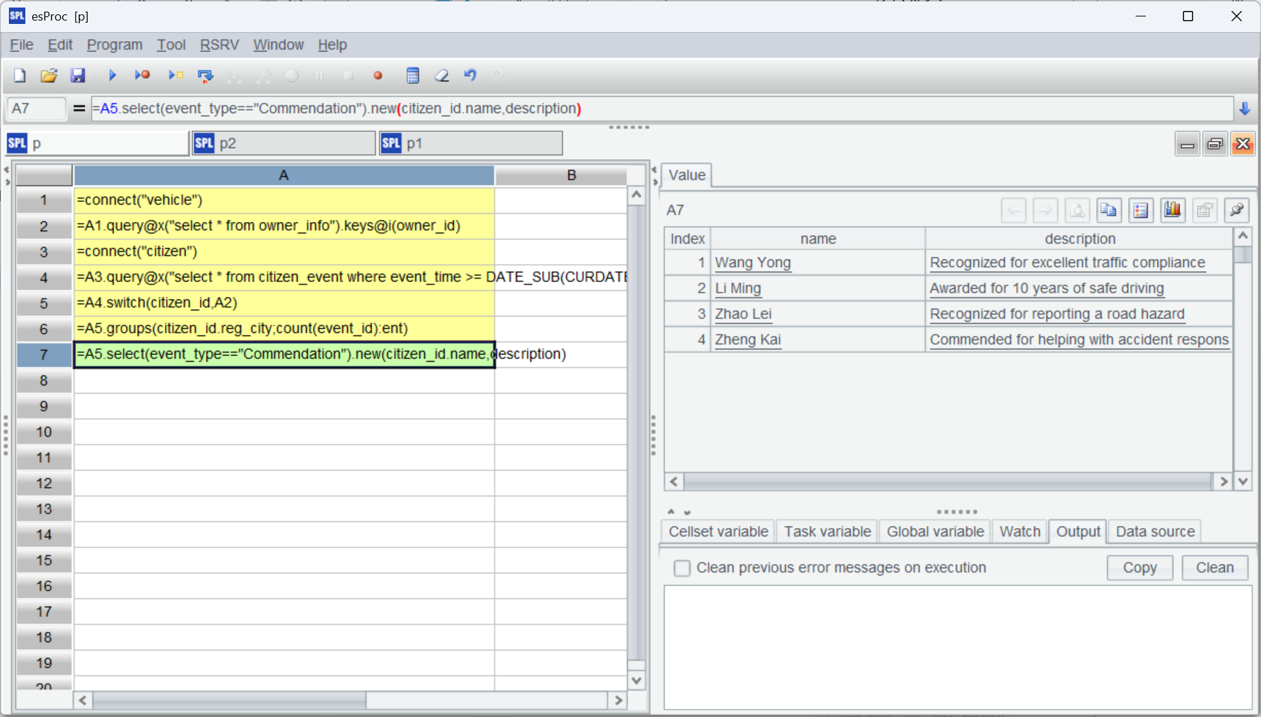
Let’s move on to another computing goal: find owners who get commended in the past year and descriptions of their events.

Add another line of code to the preceding script:

	A
…	…
7	=A5.select(event_type=="Commendation").new(citizen_id.name,description)

It performs the computation also based on A5’s joining result. This is the reuse of the joining result.

esProc’s categorizing foreign key-based joins has great advantage. In terms of coding and understanding, it is convenient to use the dot operator (.), which is similar to object.property, to reference any of the fields in any of the level of the foreign key table (dimension table may still have a dimension table) and it is easy to express the self-join and the circular reference).

When citizen_event table stores a very large amount of data, esProc can still manage. But if the data amount is too large to fit completely into the memory, recording addresses for memory data becomes infeasible because the pre-computed data addresses cannot be stored in the external memory. In that case, addresses can only be obtained while data is being retrieved.

Count personal vehicle events for each citizen having a vehicle in each city:

	A
1	=connect("vehicle")
2	=A1.query@x("select * from owner_info").keys@i(owner_id)
3	=connect("citizen")
4	=A3.cursor@x("select * from citizen_event")
5	=A4.switch(citizen_id,A2)
6	=A5.groups(citizen_id.reg_city;count(event_id):ent)

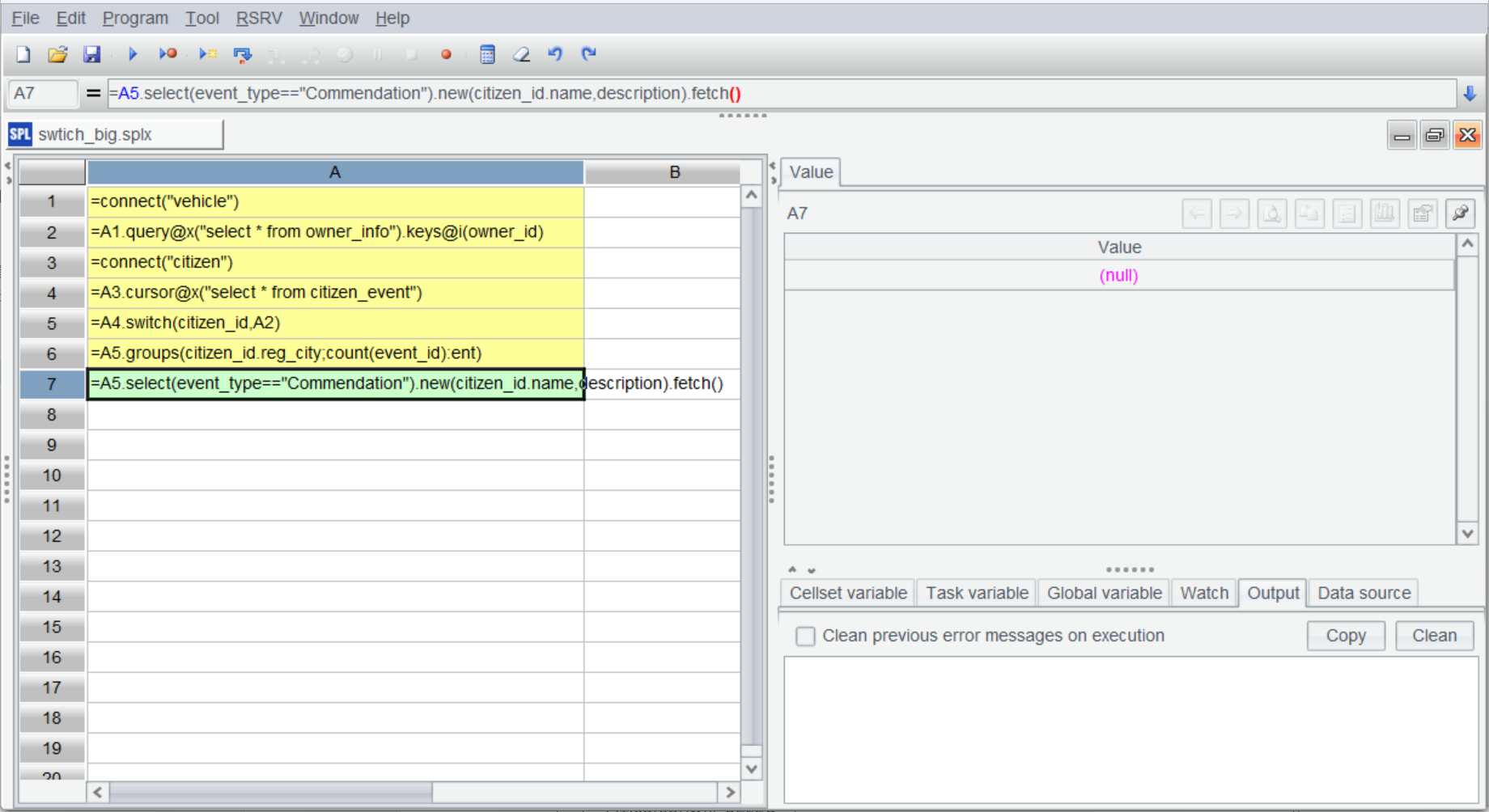
The code is mostly similar to that for the in-memory computation. The difference is that A4 uses cursor() function to create a cursor to retrieve data in batches. esProc cursors are delayed cursors, where the attached operations will only be executed when data is actually retrieved.

Cursors are a one-way mechanism. If there are more computing goals, such as finding car owners who get commended, performing computations based on A5 cannot get the desired result (like the result of A7 shown below):

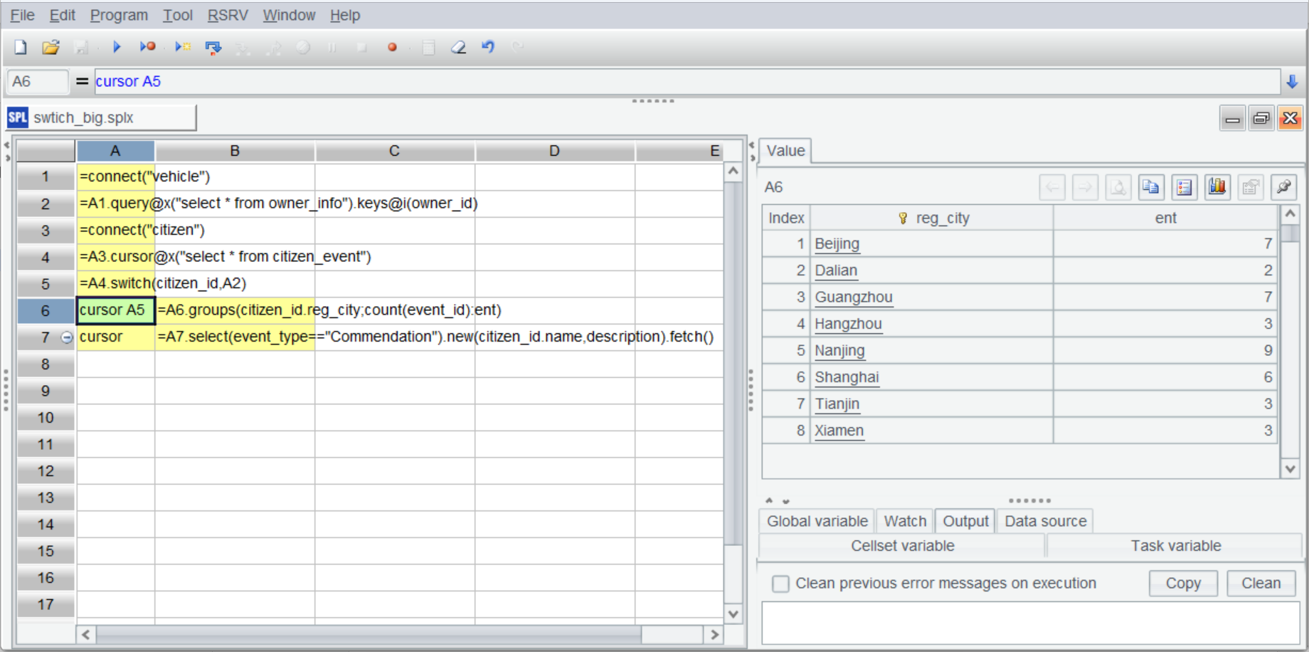
To address this error, esProc offers channel mechanism:

	A	B
1	=connect("vehicle")
2	=A1.query@x("select * from owner_info").keys@i(owner_id)
3	=connect("citizen")
4	=A3.cursor@x("select * from citizen_event")
5	=A4.switch(citizen_id,A2)
6	cursor A5	=A6.groups(citizen_id.reg_city;count(event_id):ent)
7	cursor	=A7.select(event_type=="Commendation").new(citizen_id.name,description).fetch()

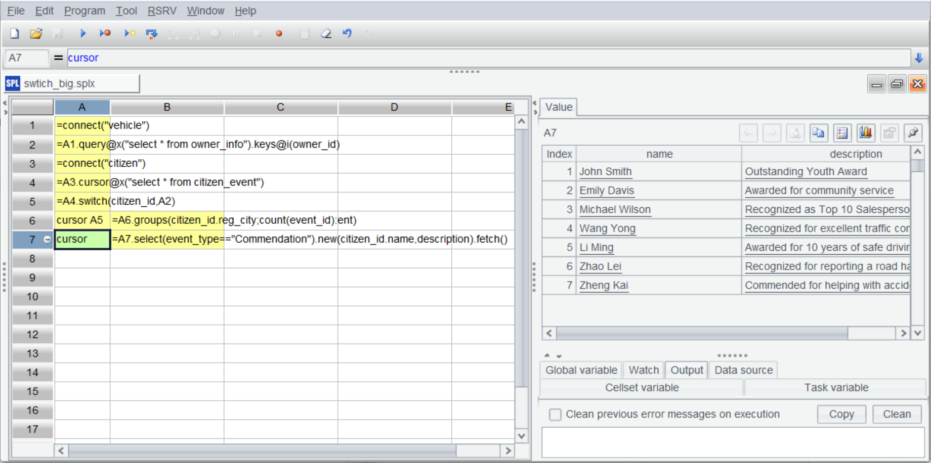
Both A6 and A7 create channels based on A5 (A7 is the simplified syntax). B6 performs grouping & aggregation based on A6’s channel and returns result to it:

B7 selects records of owners who get commended based on A7’s channel. Below is A7’s result:

Primary-subtable joins

Count the frequency of vehicles violating the traffic rules for each brand in each year.

	A
1	=connect("vehicle")
2	=A1.query@x("select * from vehicle_master")
3	=connect("traffic")
4	=A3.query@x("select * from traffic_violation")
5	=join(A2:v,plate_no;A4:t,plate_no)
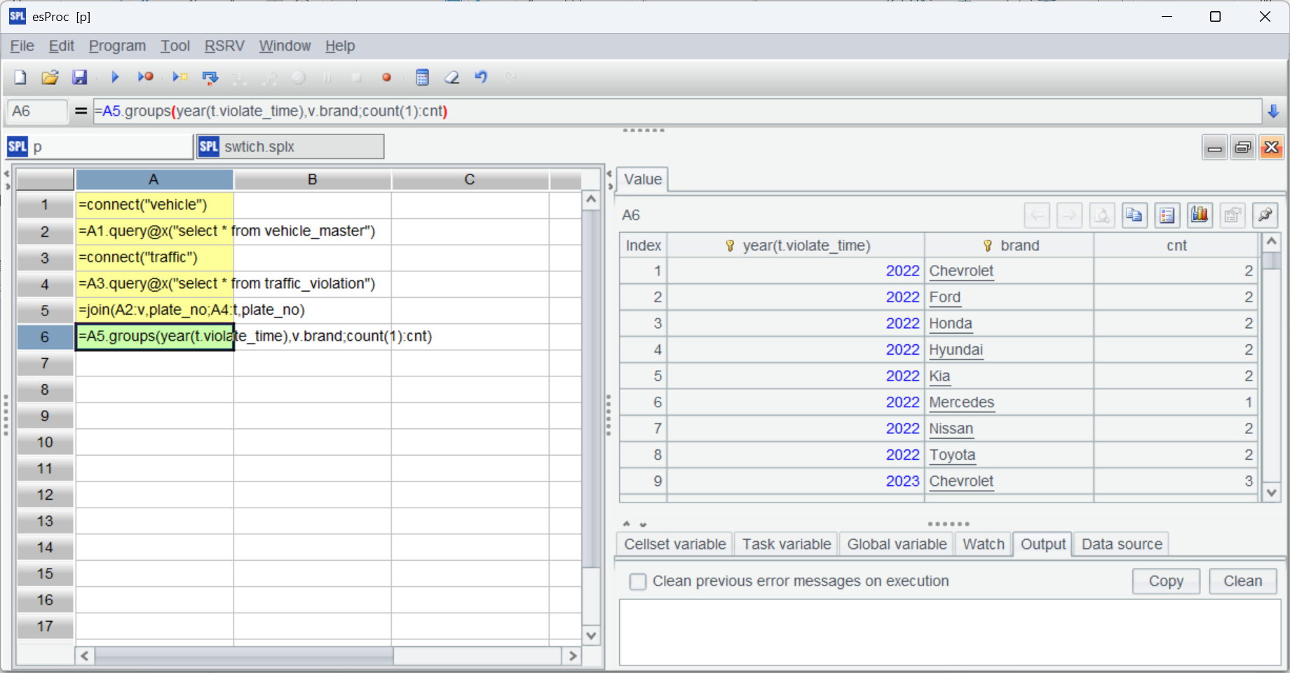
6	=A5.groups(year(t.violate_time),v.brand;count(1):cnt)

A5 uses join() function to join two tables on plate_no and returns the following result:

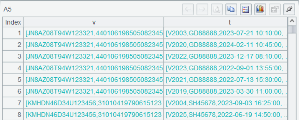
This is a multilevel set, which contains whole records of tables on both sides. Click field values of a record and we can see details as follows:

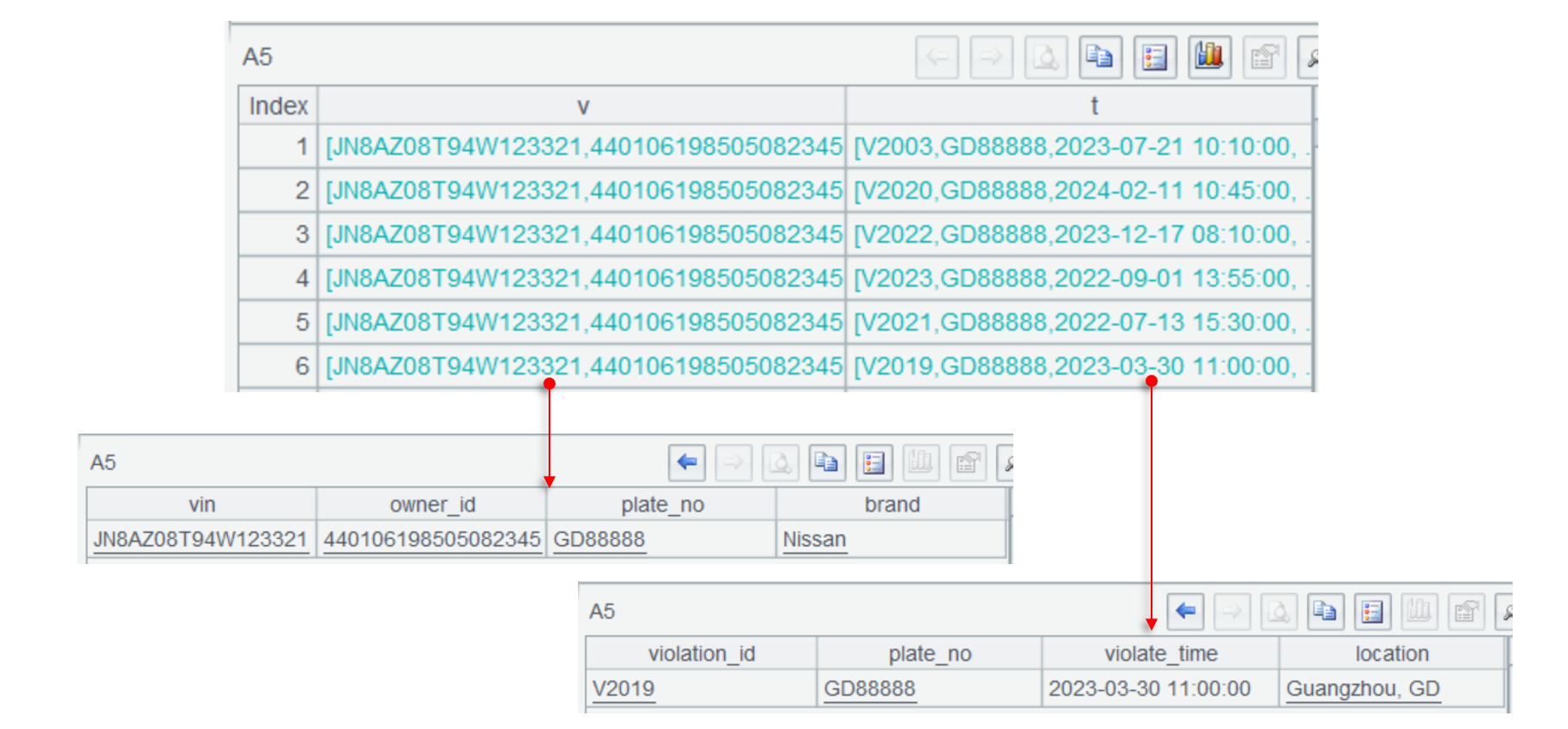
After the join is done successfully, A6 can perform grouping and aggregation through cross-level data reference.

Instead of the switch()function used in handling the foreign key-based join, join() function is used to deal with primary-subtable joins. The join() function works with different options to achieve different joining goals. @1 means a left join, @f means a full join, and @d finds the difference. The function can be also used to handle a foreign key-based join.

Then why does esProc only offers join() function to cope with both types of join operations?

The join computations in our examples involve only two tables. If there is more than one dimension table in a join computation – which is the most frequently encountered case, switch()function can be used to attach dimension tables (a dimension table may also have dimension tables) to the fact table. But it is difficult to use join() function to express the hierarchical relationships, and even you make it, coding is inconvenient.

The two tables involved in the primary-subtable join may also be very large. But we can use the ordered merge algorithm to perform the join during one traversal according to the feature that the associated fields in both tables are primary keys (or a part of the primary keys).

Count the frequency of traffic violations for each brand in each year:

	A
1	=connect("vehicle")
2	=A1.cursor@x("select * from vehicle_master order by plate_no")
3	=connect("traffic")
4	=A3.cursor@x("select * from traffic_violation order by plate_no")
5	=joinx(A2:v,plate_no;A4:t,plate_no)
6	=A5.groups(year(t.violate_time),v.brand;count(1):cnt)

A2 and A4 use cursor() function to create cursors, where the SQL statements sort records by plate_no.

In A5, joinx() function performs ordered merge and returns a cursor. The subsequent code is the same as that for handing in-memory computations.

The ordered traversal is implemented based on the feature that the associated fields are ordered. It is suitable for handle primary-subtable joins (which may be ordered by the primary key), but not fit for dealing with dimension-based foreign-key-style joins shown in the preceding example. A table may have multiple foreign key fields that are involved in the join, but it is impossible to make one table ordered by multiple fields at the same time. This is why different functions (algorithms) are designed for different types of joins.

Remember that no matter which data sources are involved, cross-database or -any-other-source, as long as the data source can be connected and accessed, the subsequent operations are always the same because SPL provides the unified data object: table sequence and cursor.