When data of the same structure is stored in different databases by year, cross-base mixed-source computation becomes inevitable for performing data analysis. Actually, no matter what sources same-structure data comes from, databases or any other storage systems, the way of performing data union is generally similar. Only the data retrieval method varies with different data sources (each of which has their own driver/corresponding function).

Setting up database connection

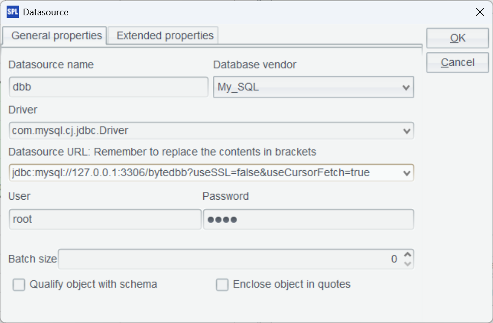
In the previous practice, we set up a database named dba. Here we set up another database named dbb. This is the connection string:

jdbc:mysql://127.0.0.1:3306/bytedbb?useSSL=false&useCursorFetch=true

Mixed-computation

First union all data coming from the two tables and then perform computations.

	A
1	=connect("dba")
2	=A1.query@x("select * from orders")
3	=connect("dbb")
4	=A3.query@x("select * from orders")
5	=A2|A4
6	=A5.groups(product_id;sum(total_amount):tamt)

A2 and A4 respectively query orders data from the two databases; @x option enables closing the database connection when the query is finished. A5 uses symbol | to union all the two sets of data. A6 performs computation (here is grouping & aggregation) based on the union result.

Execute the script and get the following result set:

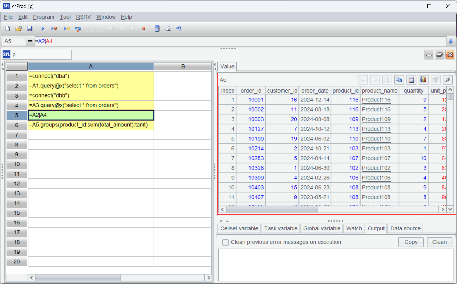
There are duplicate data between tables in the two databases, and a distinct operation is needed before performing later computations.

	A
1	=connect("dba")
2	=A1.query@x("select * from orders")
3	=connect("dbb")
4	=A3.query@x("select * from orders")
5	=A2|A4
6	=A5.group@1(order_id)
7	=A6.groups(product_id;sum(total_amount):tamt)

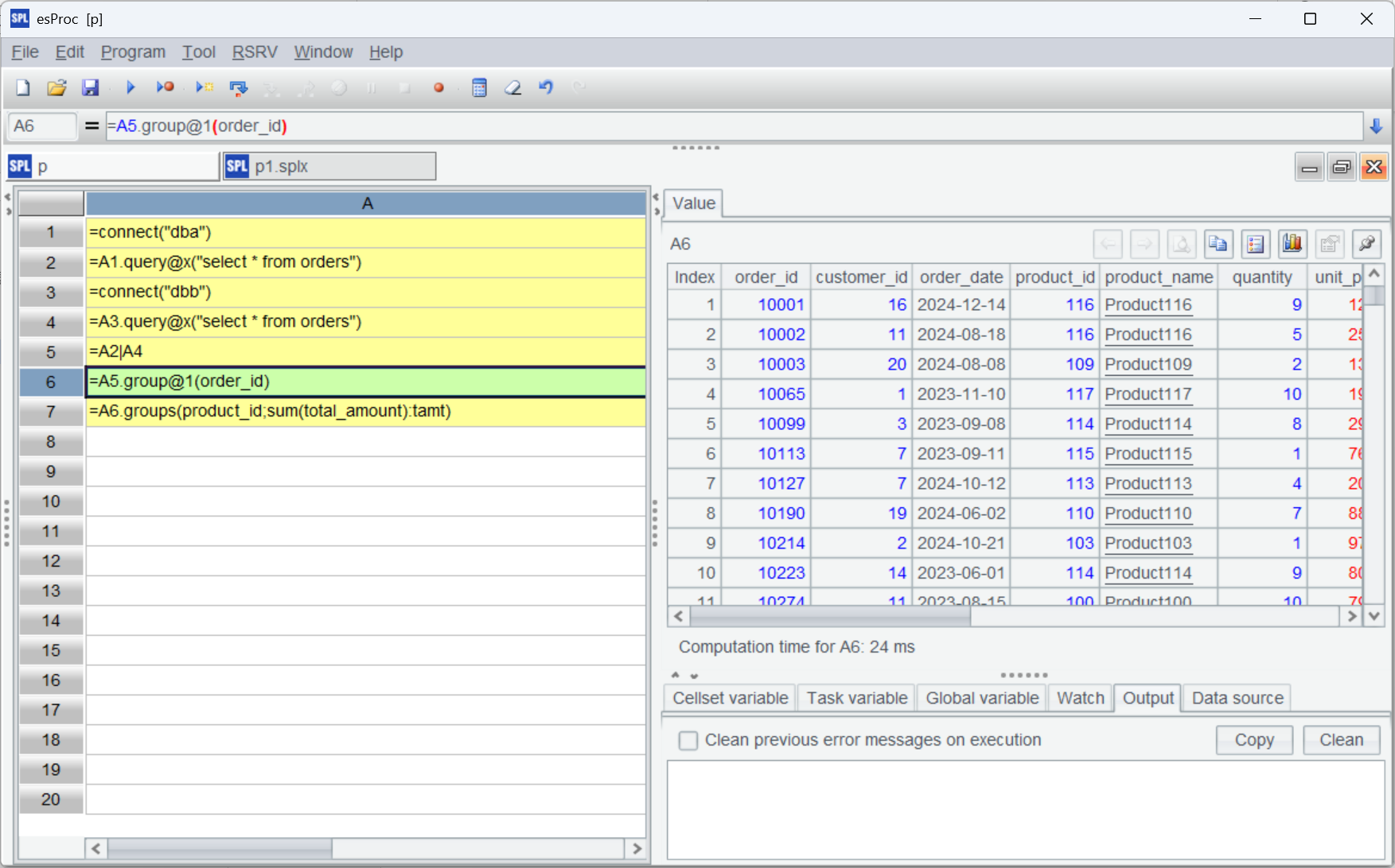
In A6, group@1 groups records by order_id and retains only the first record of each group. In this way, duplicate records are discarded. If you need to get records according to a specified condition (like getting the most recent ones), first sort the records and then perform group@1. The handling way is flexible.

View A6’s result set and we see that the duplicate records whose ids are 10001 and10002 have been removed. A7 then performs the grouping and aggregation.

The subsequent computation is the same as those for a single source table. To perform another operation, just change the expression.

Being able to perform mixed source-computations means the ability to solve data comparison problems, such as finding orders stored in both databases or those only existing in one database.

	A
1	=connect("dba")
2	=A1.query@x("select * from orders")
3	=connect("dbb")
4	=A3.query@x("select * from orders")
5	=join@f(A2:a,order_id;A4:b,order_id)
6	=A5.select(a && b)
7	=A5.select(!b).(a)
8	=A5.select(!a).(b)
9	=A5.select(a && b && (${A2.fname().("a."/~/"!=b."/~).concat("||")}))

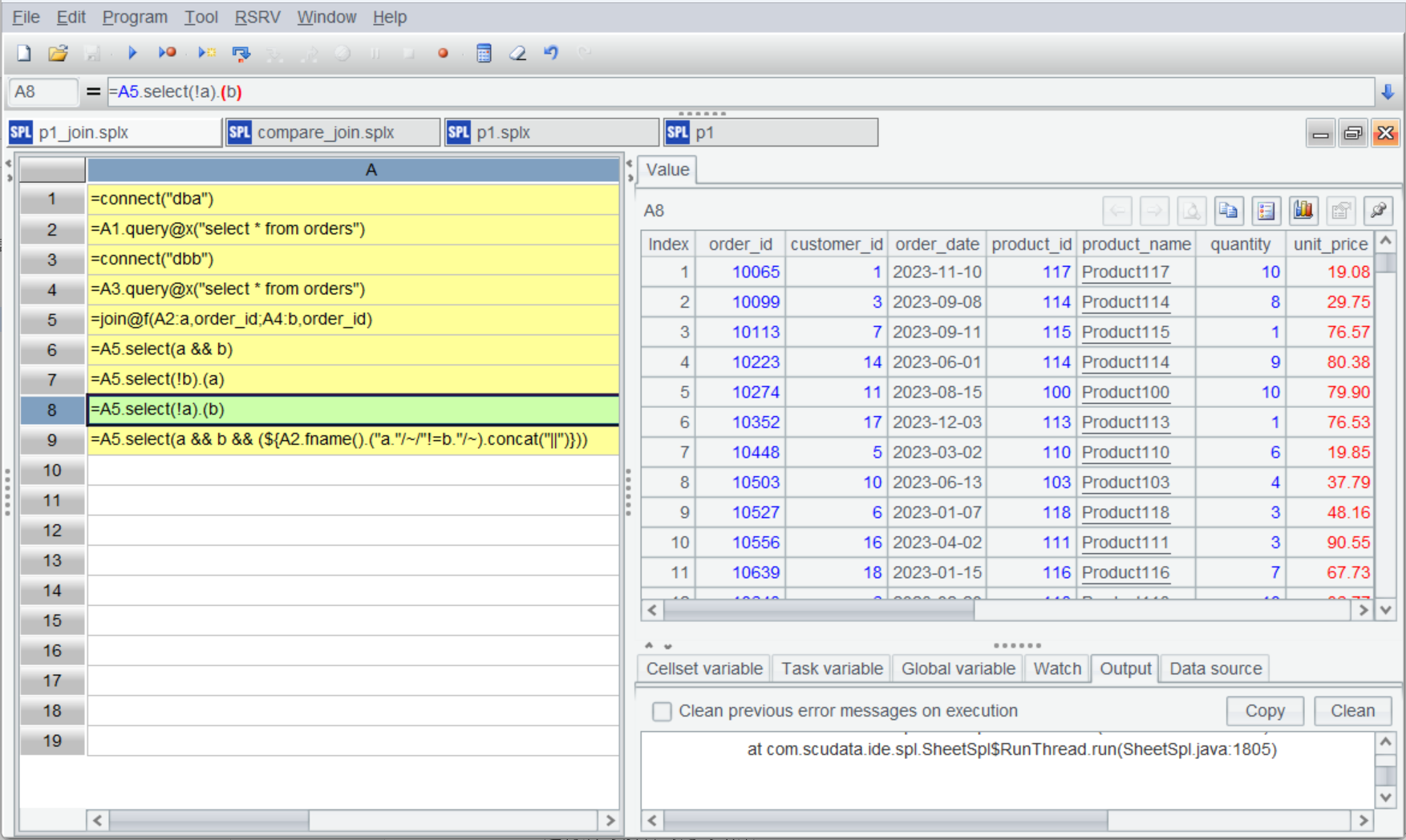
A5 uses join()function to perform a full join. A6 gets duplicate records (intersection). A7 and A8 respectively get unique records (difference). A9 gets records that have the same order_id value but that have different values in all the other fields; here macro is used to simplify the code (${A2.fname().("~(1)."/~/"!=~(2)."/~).concat("||")}). Written in a full way, it is ~(1).quantity != ~(2).quantity || ~(1).unit_price != ~(2).unit_price || ~(1).total_amount != ~(2).total_amount || ~(1).order_status != ~(2).order_status.

Execute the script and we get the following result set:

Big data handling

When data amount is large and data cannot fit into the memory, we need to use the SPL cursor mechanism to perform mixed-source computations.

When there is no need to perform a distinct operation, simply concatenate two cursors:

	A
1	=connect("dba")
2	=A1.cursor@x("select * from orders")
3	=connect("dbb")
4	=A3.cursor@x("select * from orders")
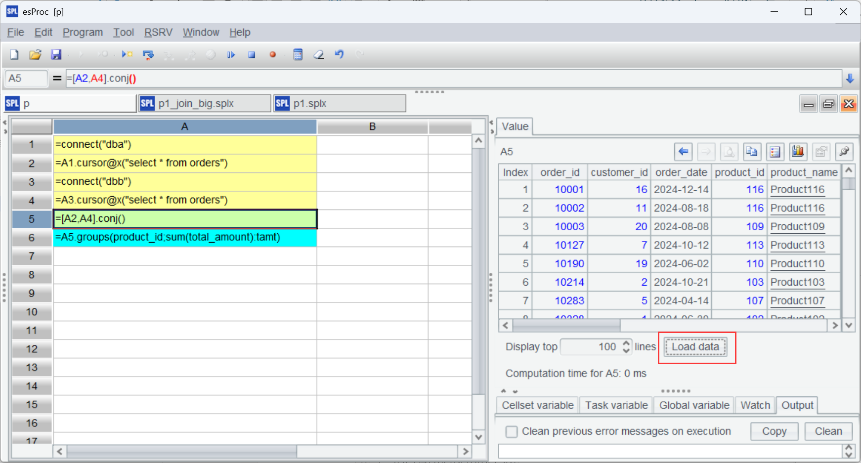
5	=[A2,A4].conj()
6	=A5.groups(product_id;sum(total_amount):tamt)

A2 and A4 use cursor() function to query data. A5 concatenates the two cursors. A6 performs grouping and aggregation. The process is generally similar to that for the whole-memory computation.

Execute the script, where A5 returns a cursor object. Click “Load data” and you can view the detailed data:

If you need to first perform a distinct operation, records in each of the cursors should be ordered in order to compare neighbors conveniently. In our example, we sort records by order_id with SQL:

	A
1	=connect("dba")
2	=A1.cursor@x("select * from orders order by order_id")
3	=connect("dbb")
4	=A3.cursor@x("select * from orders order by order_id")
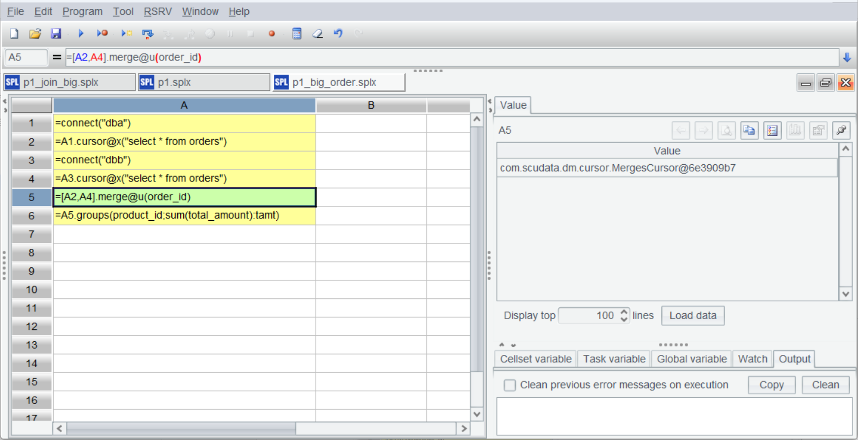
5	=[A2,A4].merge@u(order_id)
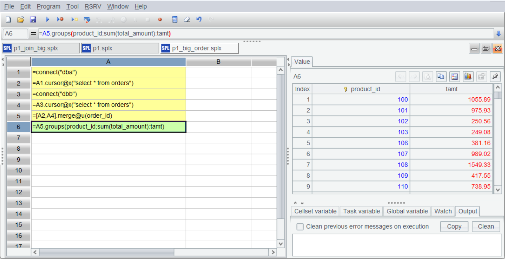
6	=A5.groups(product_id;sum(total_amount):tamt)

CS.merge() function is used to merge two ordered cursors. It has many options to work with. With @u option, it computes the union, which directly gets the unique members; with @i option, it computes the intersection; and with @d option, it gets the difference. The subsequent step of computation is the same.

The merge operation still returns a cursor (without truly performing the computation):

The computations begins and returns result at the last step of grouping and aggregation:

The overall big data handling process is basically the same as the whole-memory computation process, effectively lowering the threshold of coding in SPL.

You can also use SPL to perform big data comparison:

	A	B
1	=connect("dba")
2	=A1.query("select column_name from information_schema.columns where table_schema ='bytedba'and table_name ='orders'")
3	=A1.cursor@x("select * from orders order by 1")
4	=connect("dbb")
5	=A4.cursor@x("select * from orders order by 1")
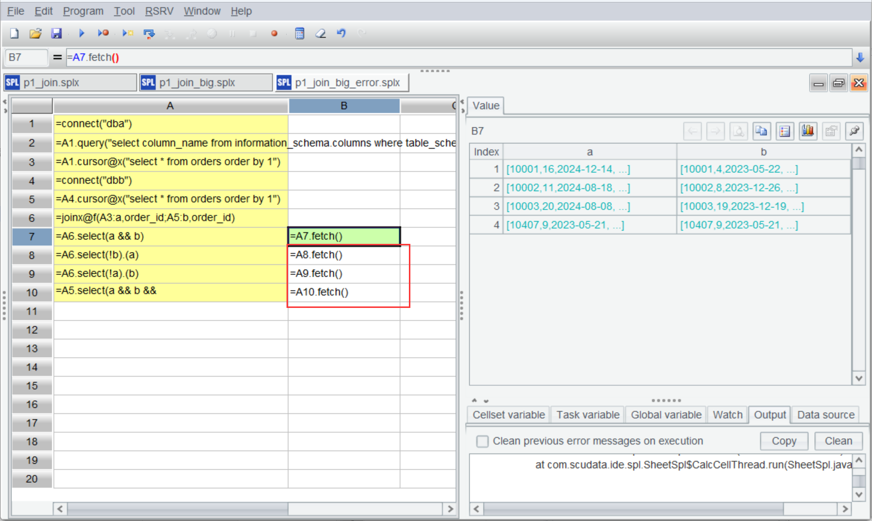
6	=joinx@f(A3:a,order_id;A5:b,order_id)
7	=A6.select(a && b)	=A7.fetch()
8	=A6.select(!b).(a)	=A8.fetch()
9	=A6.select(!a).(b)	=A9.fetch()
10	=A5.select(a && b && (${A2.(#1).("a."/~/"!=b."/~).concat("||")}))	=A10.fetch()

Since the queries in A6-A10 all return cursors, a result fetching function is used in A7-A10 to execute the computations and get results.

Strangely, only B7 has the result and cells from B8 to B10 are empty.

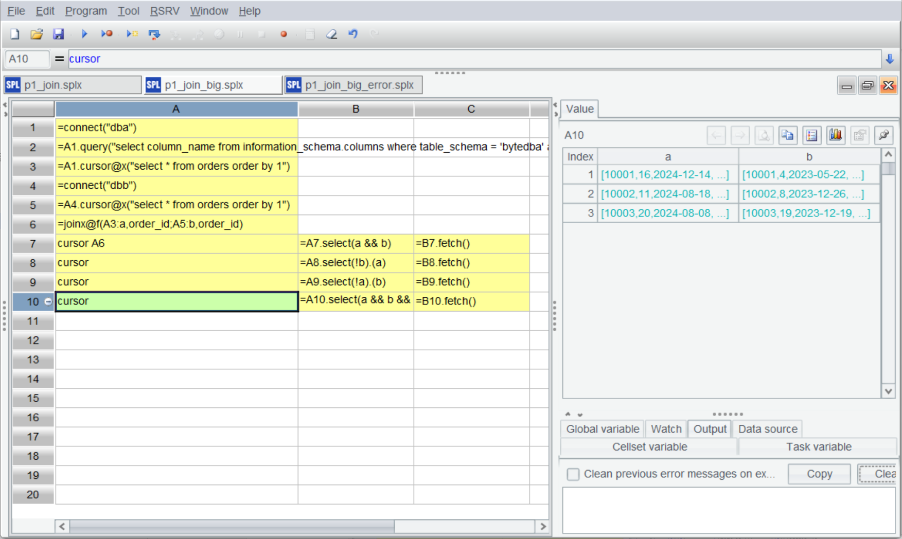
This is because the cursor is a one-way mechanism, which traverses records only once and stops. The subsequent computations thus will fail. To address this issue, we use esProc’s cursor reusing (channel) mechanism. In the big data context, multiple operations can be done during one traversal. Let’s modify the preceding code:

	A	B	C
1	=connect("dba")
2	=A1.query("select column_name from information_schema.columns where table_schema ='bytedba'and table_name ='orders'")
3	=A1.cursor@x("select * from orders order by 1")
4	=connect("dbb")
5	=A4.cursor@x("select * from orders order by 1")
6	=joinx@f(A3:a,order_id;A5:b,order_id)
7	cursor A6	=A7.select(a && b)	=B7.fetch()
8	cursor	=A8.select(!b).(a)	=B8.fetch()
9	cursor	=A9.select(!a).(b)	=B9.fetch()
10	cursor	=A10.select(a && b && (${A2.(#1).("a."/~/"!=b."/~).concat("||")}))	=B10.fetch()

A7-A10 create channels based on A6’s channel (A8-A10 are simplified syntax). Computations in B7-C10 are the same as those in the preceding cellset. After the script is executed, results can be viewed in A7-A10 (Note: not in C7-C10):

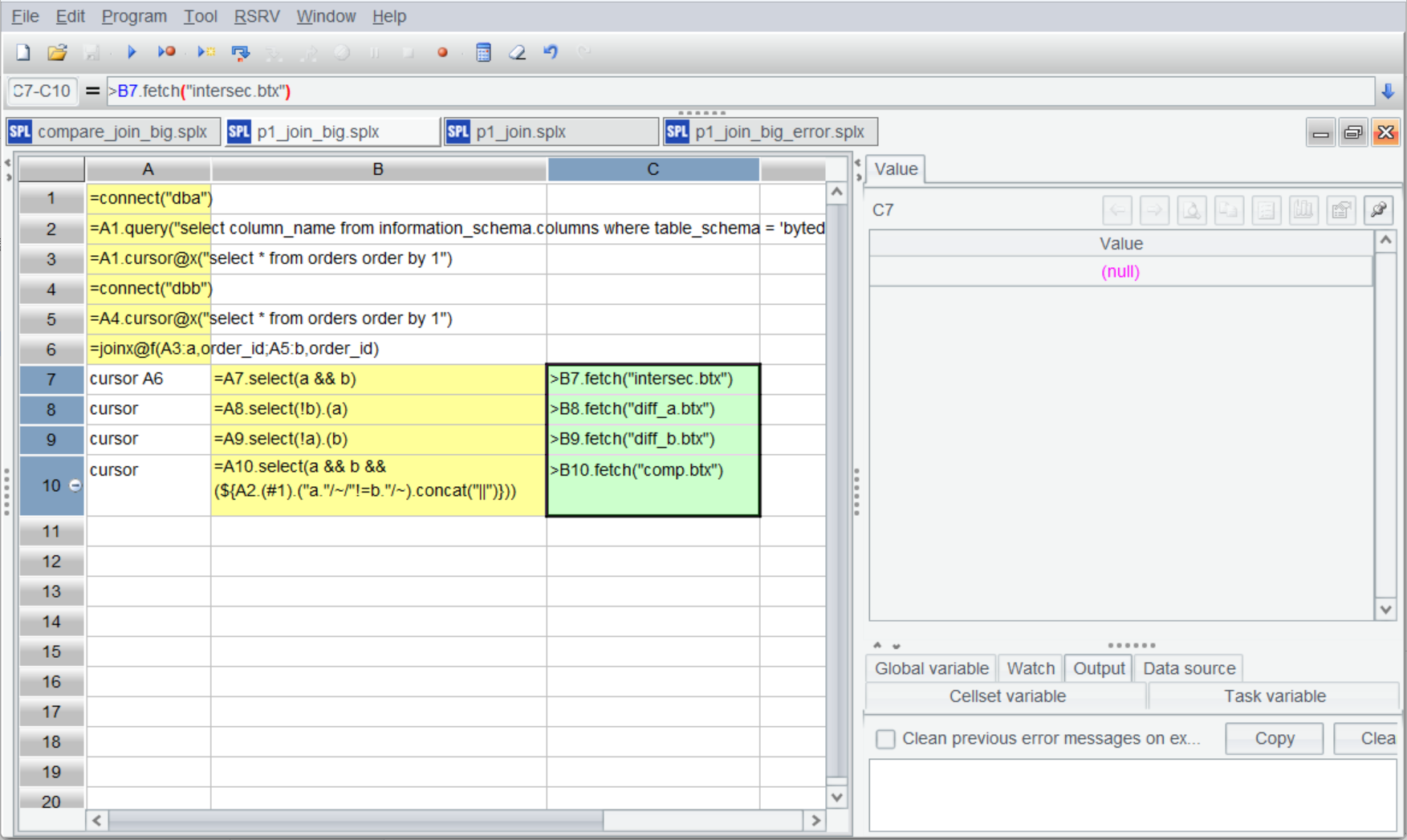
If the results are still too large to fit into the memory, you can export them to files. Modify the preceding code as follows:

	A	B	C
1	=connect("dba")
2	=A1.query("select column_name from information_schema.columns where table_schema ='bytedba'and table_name ='orders'")
3	=A1.cursor@x("select * from orders order by 1")
4	=connect("dbb")
5	=A4.cursor@x("select * from orders order by 1")
6	=joinx@f(A3:a,order_id;A5:b,order_id)
7	cursor A6	=A7.select(a && b)	>B7.fetch("intersec.btx")
8	cursor	=A8.select(!b).(a)	>B8.fetch("diff_a.btx")
9	cursor	=A9.select(!a).(b)	>B9.fetch("diff_b.btx")
10	cursor	=A10.select(a && b && (${A2.(#1).("a."/~/"!=b."/~).concat("||")}))	>B10.fetch("comp.btx")

A file to which the result will be exported is added to fetch() function in each cell of C7-C10.

Execute the script and get the following result files:

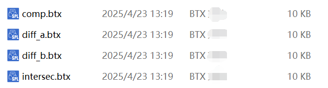
It is easy for SPL to deal with any cross-database/cross-source computing goals.