There are also some other commonly seen data sources, including NoSQL, MQ, MongoDB and others, among which MongoDB is the most commonly used. Now let’s use SPL to connect to MongoDB for computations.

Import data from the MongoDB.

External library

Data sources SPL supports can be generally divided into two categories. One category includes RDBs, which can be accessed through JDBC, and files, from which data can be directly retrieved. The other covers non-relational data sources such as MongoDB, which are simply encapsulated by SPL based on their official driver jars and provided in the form of external library.

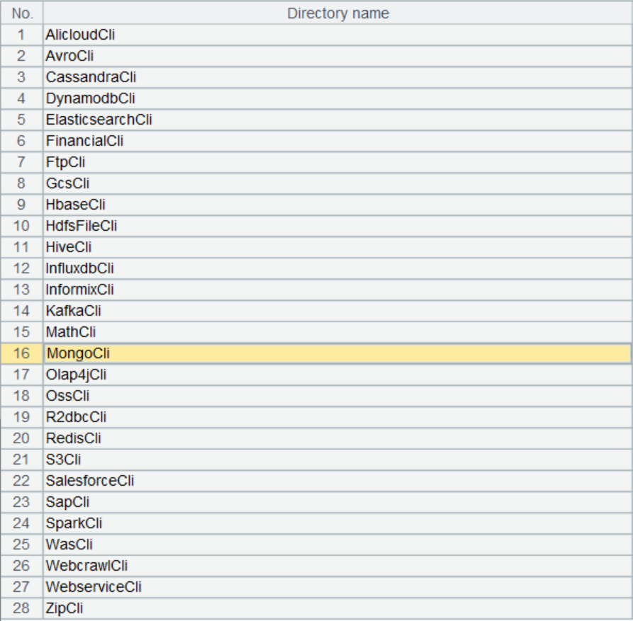
SPL external library contains dozens of non-relational data sources and functions:

External connectors are placed in the external library, which is the external function extension library. Submitting specialized functions, which are used infrequently in handling the commonly seen computing problems, in the form of external library lets users load them off-the-cuff when needed.

There are a large variety of external data sources. Not all of them are frequently used. Providing these external connectors in the form of external library is more flexible, allowing new data sources added to the library without affecting the existing sources.

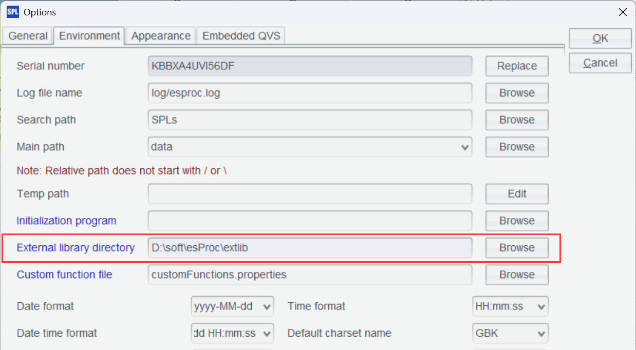
To use the external library, first you need to download the external library driver.

Put the driver in any directory, such as [installation directory] \esProc\extlib, and load that external library directory in IDE and check the external library item you need.

Computing use case

The set Orders stores order-related information. Its structure and content are as follows:

{
  "_id": {
    "$oid": "6826ade0cbc0428d8335b0bb"
  },
  "order_id": "ORD1001",
  "customer": "C001",
  "order_date": {
    "$date": "2025-01-15T00:00:00.000Z"
  },
  "order_details": [
    {
      "product_id": "P001",
      "product_name": "Laptop",
      "quantity": 1,
      "price": 899.99
    },
    {
      "product_id": "P005",
      "product_name": "Wireless Mouse",
      "quantity": 2,
      "price": 19.99
    }
  ]
}

Find customers whose order amounts rank in top 3.

SPL script:

	A
1	=mongo_open("mongodb://127.0.0.1:27017/raqdb")
2	=mongo_shell@d(A1,"{'find':'orders'}")
3	=A2.groups(customer; order_details.sum(quantity*price):amount)
4	=A3.top(3,-amount)

A1: Connect to MongoDB.

A2: Query orders data. @d enables returning result as a table sequence.

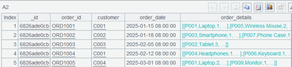
This is a multilevel result set, where order_details can be expanded. It is similar to the JSON data handled in the preceding practice.

A2 executes a command that uses purely native MongoDB syntax. Now execute the command on MongoDB Shell:

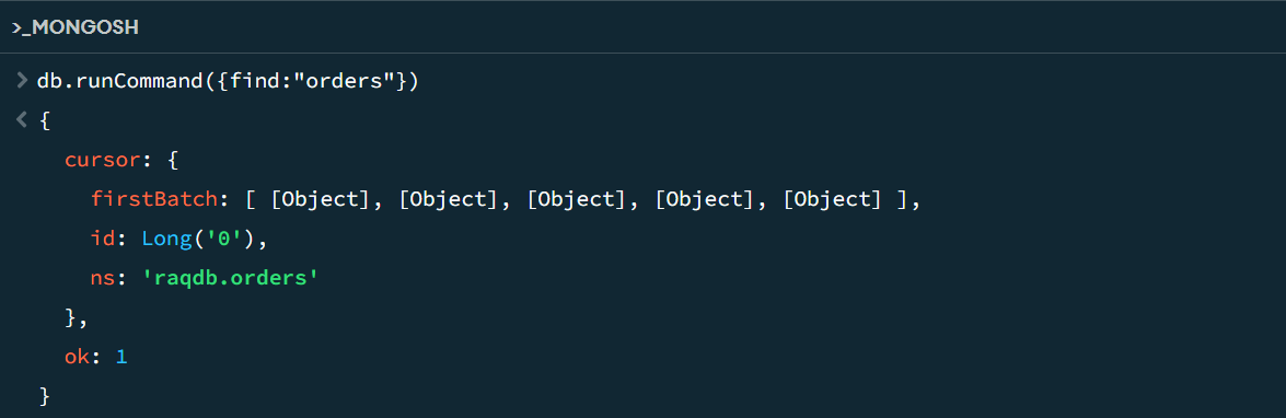
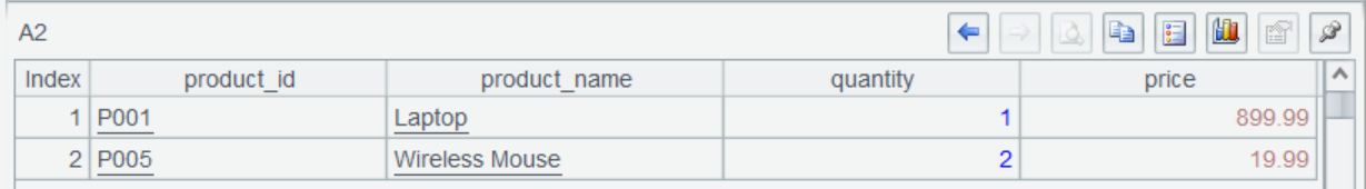
The command successfully returns a cursor. From the cursor we fetch one record:

Group A2’s records and sum order amounts by customer. The subsequent computations are the same.

A4: Use top() function to get top 3 customers.

Let’s perform another filtering to get orders before 2025-02-01.

Modify A2 as:

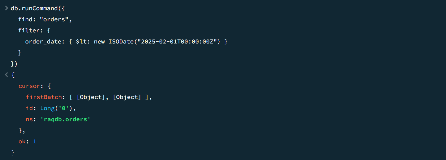
=mongo_shell@d(A1,"{'find':'orders',filter: {order_date: { $lt: new ISODate('2025-02-01T00:00:00Z') } }}")

And get the following result:

Execute the same command in MongoDB and you can get the same result:

Now we have taken MongoDB to illustrate the SPL way of handling non-relational data sources. The way also applies to handling the other data sources. Just set up the external library and use the corresponding native SPL syntax to access it.

To access Kafka, for example:

	A
1	=kafka_open("/kafka/my.properties", "topic1")
2	=kafka_poll(A1)
3	=A2.derive(json(value):v).new(key, v.fruit, v.weight)
4	=kafka_close(A1)

To access Elasticsearch:

	A
1	>apikey="Authorization:ApiKey a2x6aEF……KZ29rT2hoQQ=="
2	'{"counter": 1,"tags": ["red"] ,"beginTime":"2022-01-03","endTime":"2022-02-15"}
3	=es_rest("https://localhost:9200/index1/_doc/1", "PUT",A2;"Content-Type: application/x-ndjson",apikey)
4	=json(A3.Content)

To access HDFS:

	A
1	=hdfs_open("hdfs://192.168.0.8:9000", "root")
2	=hdfs_file(A1,"/user/root/orders.txt":"UTF-8")
3	=A2.read()
4	=A2.import@t()

SPL’s “native driver + simple encapsulation” way is simple and convenient. It helps retain characteristics of the data source and make good use of its storage and computing capabilities, and enables direct access without performing “some” data loading operation. It is also easy for users to add more data sources. But since SPL directly writes the data accessing code in the script and uses the native driver, you need to modify the script when the data source is changed. This means SPL is not as transparent to the low-level data source as logical data warehouses to the data source.

Logical data warehouses use special connectors to connect to corresponding data sources, achieving complete transparency to the low-level layer. For each type of data source, the connector needs to be specifically developed. The development is very complicated, and, as a result, the available connectors are limited. It is also difficult for users to make further development based on the open-source code; usually they can only wait for vendor’s provision.

The special connectors logical warehouses use and SPL’s native drive plus simple encapsulation method each have their advantages. The former gives in-depth support and optimization to achieve transparency to some extent. The latter is more flexible, supports more types of data sources, and makes it easy to add more. You should choose the appropriate one to meet the needs.

Now we’ve learned how to use SPL to query RDBs, CSV/XLS files, Restful/JSON data and MongoDB. Then you can connect to them and perform mixed-source computations