In data analysis applications, multi-table JOIN operations within a database often involve complex SQL and exhibit suboptimal JOIN performance. As a result, multiple tables are often joined to a wide table. For example, the orders table and several dimension tables in the figure below are likely to be converted into a wide table:

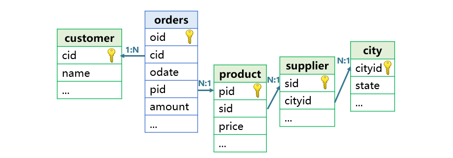
However, wide tables pose many issues: significant data redundancy, non-compliance with normalization requirements (prone to errors), and the need to update the entire wide table when dimension table data changes. Moreover, the computational performance of wide tables isn’t necessarily better than that of multi-table joins.

esProc specifically designs a sequence number-based association method, which significantly improves JOIN performance, thereby avoiding using wide tables.

In the following analysis, we take the orders table and multiple dimension tables as an example to compare the performance of the esProc multi-table approach and the MySQL multi-table and wide-table approaches. The orders table is a fact table containing ten million records. Other tables are dimension tables with relatively small data.

Test environment: VMware virtual machine with the following specifications: 8-core CPU, 8GB RAM, SSD. Operating system: Windows 11. MySQL version: 8.0.

First, download esProc at https://www.esproc.com/download-esproc/. The standard version is sufficient.

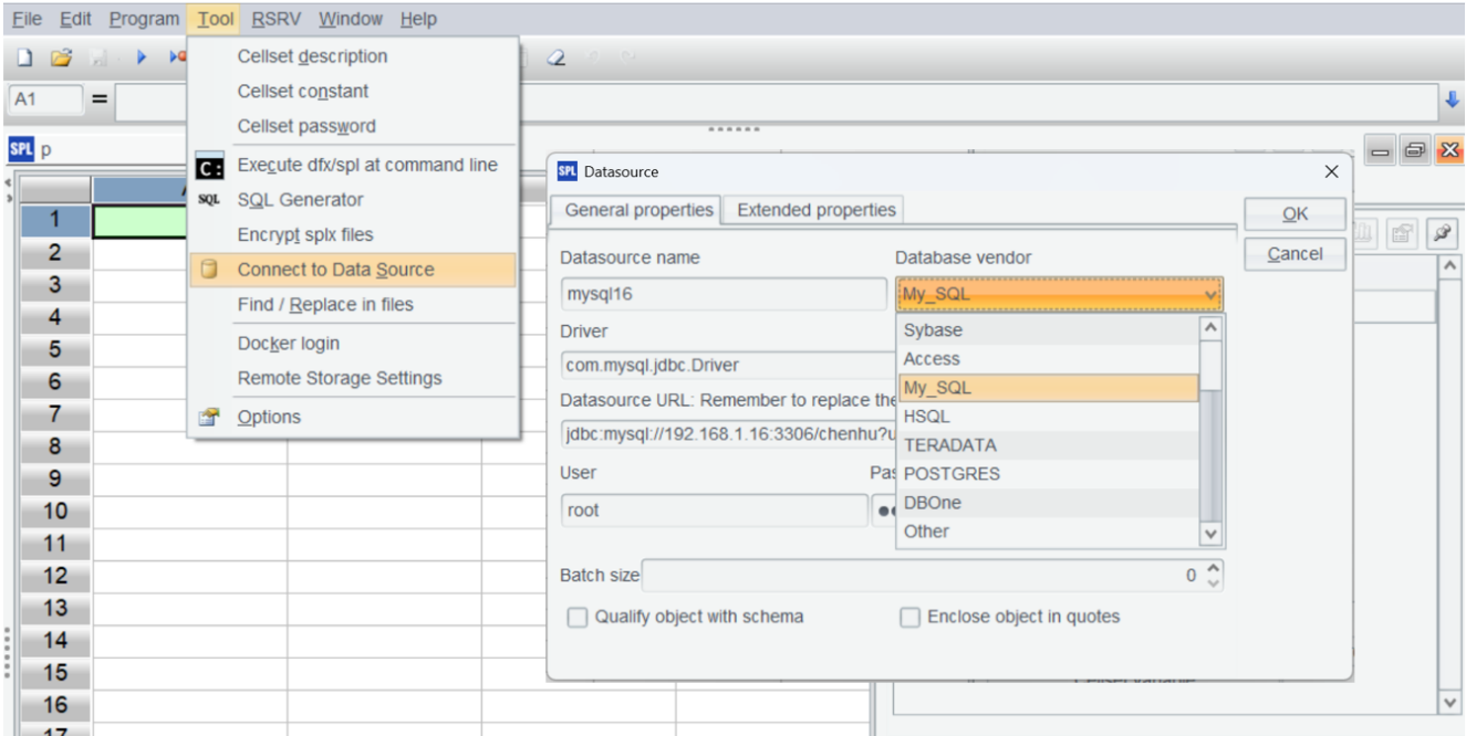
After installing esProc, test whether the IDE can access the database normally. First, place the JDBC driver of the MySQL database in the directory ‘[Installation Directory]\common\jdbc,’ which is one of esProc’s classpath directories.

Establish a MySQL data source in esProc:

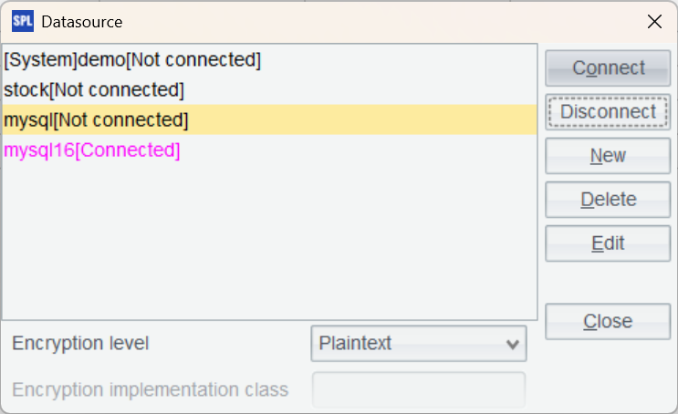
Return to the data source interface and connect to the data source we just configured. If the data source name turns pink, the configuration is successful.

Create a new script in the IDE, write SPL statements to connect to the database, and execute a SQL query to load data from the city table:

	A	B
1	=connect("mysql16")
2	=A1.query("select * from city")

Press Ctrl+F9 to execute the script. The result of A2 is displayed on the right side of the IDE, which is very convenient.

Next, prepare the data by exporting the historical data from the database to esProc’s high-performance files.

	A
1	=connect("mysql16")
2	=A1.query("select * from city").keys@i(cityid)
3	=file("city.btx").export@b(A2)
4	=A1.query("select * from supplier").keys@i(sid)
5	=file("supplier.btx").export@b(A4.new(sid,sname,A2.pfind(cityid):cityid))
6	=A1.query("select * from customer").keys@i(cid)
7	=file("customer.btx").export@b(A6)
8	=A1.query("select * from product").keys@i(pid)
9	=file("product.btx").export@b(A8.new(pid,pname,ptype,A6.pfind(sid):sid))
10	=A1.cursor("select * from orders")
11	=A10.new(oid,A6.pfind(cid):cid,A8.pfind(pid):pid,odate,amount)
12	=file("orders.ctx").create@y(oid,cid,pid,odate,amount)
13	=A12.append(A11)
14	>A1.close(),B12.close()

A2-A9 take all dimension tables. Because the dimension tables have small data volumes, storing them in bin files (btx) is convenient. The cityid field of the supplier table and the sid field of the product table need to be converted to the position number in the corresponding dimension table using the pfind function.

Since the fact table orders is large, a database cursor is created in A10.

A11 uses the pfind function to convert the cid and pid fields to the position numbers in the corresponding dimension tables.

A12 creates a composite table, and A13 writes the data from the A11 cursor into the composite table.

Here, esProc converts the dimension fields cid and pid in the fact table orders to position numbers in the dimension tables, achieving sequence-numberization. During computation, the dimension tables are pre-loaded into memory and associated. Then, the fact table data is read into memory in batches, and the records at the corresponding positions in the in-memory dimension tables are directly accessed using the dimension field values (i.e., the dimension table positions), resulting in fast processing.

The cityid and sid dimension fields in the supplier and product also need to be converted to position numbers.

After data preparation, the esProc system needs to be initialized by pre-loading the dimension table data into memory and associating the tables:

	A	B
1	=file("customer.btx").import@b()	=env(customer,A1)
2	=file("product.btx").import@b()	=env(product,A2)
3	=file("supplier.btx").import@b().keys@i(sid)	=env(supplier,A3)
4	=file("city.btx").import@b().keys@i(cityid)	=env(city,A4)
5	=supplier.run(cityid=city(cityid))	=product.run(sid=supplier(sid))

A1 to B4: Read the data of each dimension table and store them in global variables.

A5: Associate the supplier table with the city table. Since the cityid field in supplier has already been sequence-numbered, its values directly correspond to records in city, enabling the direct retrieval of records in city corresponding to the position numbers. B5: Associate the product table with the supplier table using the same position method.

After association, the sid field in the product table is assigned the value of the supplier’s record object, and the cityid field in the supplier table is assigned the value of the city’s record object.

After initialization, esProc can be used in place of a wide table for queries. For example, to group orders from suppliers in Chicago by customer and calculate the total amount, with results including customer names:

	A
1	=file("orders.ctx").open()
2	=A1.cursor@m(oid,cid,pid,amount;cid:customer:#,pid:product:#)
3	=A2.select(pid.sid.cityid.cityname=="Chicago").groups(cid;cid.cname,sum(amount):total)
4	>A1.close()

In A2, cid:customer:# means that the association between orders and customers is performed using the position number # on the cursor. After association, the cid and pid fields are converted to the record objects of the corresponding tables.

Computation in A3 becomes easier, enabling code to be expressed using object property notation, such as pid.sid.cityid.cityname.

The actual execution time of this script is 1.3 seconds.

The @m in A2 means that multi-threaded computation is enabled according to the parallel option configured in Options.

This parallel option needs to be enabled.

SQL for MySQL multi-table approach:

SELECT c.cid,c.cname,SUM(o.amount)
FROM 
    orders o
JOIN 
    customer c ON o.cid = c.cid
JOIN 
    product p ON o.pid = p.pid
JOIN 
    supplier s ON p.sid = s.sid
JOIN 
    city ci ON s.cityid = ci.cityid
WHERE 
    ci.cityname = 'Chicago'
GROUP BY 
    c.cid, c.cname

Execution time: 28 seconds.

SQL for MySQL wide-table approach:

SELECT cid,cname,SUM(amount)    
FROM 
    orders_all 
WHERE 
    cityname = 'Chicago'
GROUP BY 
cid, cname

Execution time: 33 seconds.

This code is simpler than that of multi-table join, but the performance decreases. This may be because the wide table has more columns, requiring more data to be read during computation, which slows down the process.

Let’s look at another calculation: group orders by supplier and count the orders in each group, with results including the supplier’s name and city. Based on the previous esProc SPL code in A2, various calculations can be easily implemented by simply modifying the A3 code.

=A2.groups(pid.sid;pid.sid.sname,pid.sid.cityid.cityname,count(1))

Execution time: 1 second.

MySQL multi-table approach:

SELECT s.sid,s.sname,c.cityname,COUNT(o.oid)
FROM 
    orders o
JOIN 
    product p ON o.pid = p.pid
JOIN 
    supplier s ON p.sid = s.sid
JOIN 
    city c ON s.cityid = c.cityid
GROUP BY 
s.sid, s.sname, c.cityname, c.statename;

Execution time: 36 seconds.

MySQL wide-table approach:

SELECT sid,sname,cityname,statename,count(oid)
FROM 
    orders_all
GROUP BY 
    sid, sname, cityname, statename

Execution time: 44 seconds.

Test results:

	MySQL multi-table	MySQL wide table	esProc
Computation 1	28 seconds	33 seconds	1.3seconds
Computation 2	36 seconds	44 seconds	1 second

The computing performance of esProc multi-table join significantly surpasses that of MySQL multi-table and wide-table approaches, and the SPL code is much simpler, completely avoiding wide tables.

When preparing data, exporting data from the database is time-consuming, but since this is a one-time operation, the longer duration is acceptable. When the orders table has incremental data in the future, you only need to append the new data to the composite table on a regular basis.

However, when the data of dimension tables changes, it will be a bit cumbersome, as they require regenerating the btx files and reloading them into memory. Moreover, because the result of sequence-numberization of the fact table relies on the record order in the dimension tables, any changes to the dimension tables (like adding or deleting records) necessitate a complete regeneration of the fact table, leading to a relatively high maintenance and management cost.

In practice, numerous computational scenarios are based on the static historical data, and many multi-table join scenarios require urgent performance improvements. For these scenarios, the SPL sequence-number association method can effectively speed up multi-table joins, thereby avoiding wide tables.