The following is part of the data from the simplified purchases table ‘purchases’ and sales table ‘sales’:

sales:

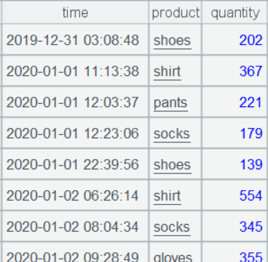
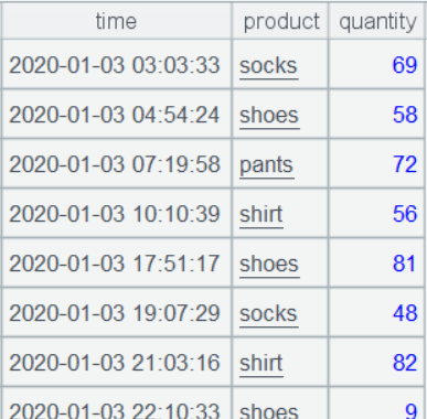
purchases:

Download test data

1. Calculate the number of weeks each product experienced stock-out

It is required to count only the week in which a product becomes stock-out; if a product remains stock-out for multiple consecutive weeks, subsequent weeks are excluded from the count.

The approach to solving this problem is as follows: First, treat purchases as inventory increases and sales as inventory decreases. Therefore, we convert the sales quantities to negative numbers. Next, union the two tables and sort by product and time. This unions the purchase and sales quantities together. Then, calculate the cumulative sum sequentially — when the sum reaches 0, a stock-out event occurs. Restart the cumulative sum when encountering a new product. Since a product may experience multiple stock-out events within a single week, direct counting of these events would lead to duplicates. To avoid this, set all stockout timestamps to their corresponding Mondays and then deduplicate and count.

Let’s look at the SQL code first:

with t1 as (
  select time,product,-quantity quantity from sales
  union all
  select * from purchases
),
t2 as (
  select *, 
  sum(quantity) over(partition by product order by time) cum
  from t1
)
select product, count(distinct date_sub(date(time), interval weekday(time) day)) cnt
from t2
where cum=0
group by product;	

First uses a subquery to merge the two tables.

Due to the unordered nature of SQL sets, the order of results from a subquery cannot be leveraged for subsequent cumulative calculations. As a result, the operations – grouping, in-group sorting, and accumulating – need to be performed within a single window function, which requires a second subquery.

In contrast, SPL sets are ordered; during multi-step calculations, the order is kept for subsequent steps. The cum() function can perform in-group accumulation on ordered sets, making it directly usable in conditions for filtering stock-out records. The pdate() function can obtain various special dates, including the Monday used here.

	A
1	=file("purchases.txt").import@t()
2	=file("sales.txt").import@t().run(quantity=-quantity)
3	=(A1|A2).sort(product, time)
4	=A3.select(cum(quantity;product)==0)
5	=A4.groups(product;icount(pdate@w1(time)):cnt)

A1: Load the purchases; A2: Load the sales and convert the quantity to negative numbers.

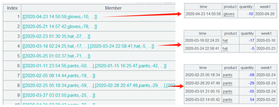
SPL IDE is highly interactive, allowing for step-by-step execution and easy visual inspection of the results of each step in the right-hand panel at any time. A3 uses | to union the two tables, and sort by product and time. Select A3, the result data will be displayed on the right:

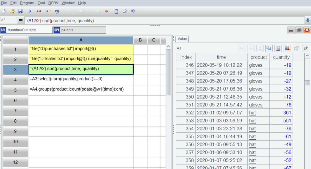
A4: Filter stock-out records where the cumulative sum for each product is 0.

A5: When counting quantities by product on Monday, the icount() function performs deduplicating and counting.

Once you are familiar with SPL, these calculation steps can be simply written in one statement:

	A
1	=file("purchases.txt").import@t()
2	=file("sales.txt").import@t().run(quantity=-quantity)
3	=(A1|A2).sort(product, time) .select(cum(quantity;product)==0) .groups(product;icount(pdate@w1(time)):cnt)

2. Calculate the time periods of stock-out weeks for each product

Use the method described in the previous problem to find the Monday dates for all stock-out weeks of each product. Sort these dates, and then group them by consecutive weeks (where the interval between Mondays is either 0 or 7 days). The period from the Monday of the first week to the Sunday of the last week represents the time period of this group of consecutive stock-out weeks.

SQL:

with recursive t1 as (
  select time,product,-quantity quantity from sales
  union all
  select * from purchases
),
t2 as (
  select *, sum(quantity) over(partition by product order by time) cum
  from t1
),
t3 as (
  select product, date_sub(date(time), interval weekday(time) day) week1
  from t2
  where cum=0
),
t4 as (
  select *, row_number() over(partition by product order by week1) rn
  from t3
),
t5 as (
  select product, min(week1) start, min(week1) week1, rn
  from t4 
  group by product
  union all
  select h.product, (case when datediff(h.week1,q.week1)>7 then h.week1 else q.start end), h.week1, h.rn
  from t4 h join t5 q
    on h.product=q.product and h.rn=q.rn+1
)
select product, concat(start, ',', max(week1)+interval 6 day) segment
from t5
group by product,start
order by product,start;

SQL sets are unordered and do not support accessing records by position. When comparing with the previous record, you first need to use a subquery t4 to add a row number rn. Then, in t5, self-join t4 and use the condition h.rn=q.rn+1 to reference adjacent rows. Additionally, since there are multiple consecutive comparisons, a recursive subquery must be specified. Originally, the goal was simply to check if the weeks of two consecutive dates are continuous, but the approach of assigning row numbers and recursively joining has become overly complicated.

SPL’s ordered sets allow referencing data by position, making it easy to check if weeks are consecutive. In addition to the most common equi-grouping, SPL also supports conditional grouping, enabling code to be written in a completely natural way:

	A
1	=file("purchases.txt").import@t()
2	=file("sales.txt").import@t().run(quantity=-quantity)
3	=(A1|A2).sort(product, time)
4	=A3.select(cum(quantity;product)==0).derive(pdate@w1(time):week1)
5	=A4.group@i(product!=product[-1] || week1- week1 [-1]>7)
6	=A5.new(product, ~1.week1/","/(~.m(-1).week1+6):segment)

A4: Calculate the date of Monday for each stock-out week, while preserving the order of A3 set.

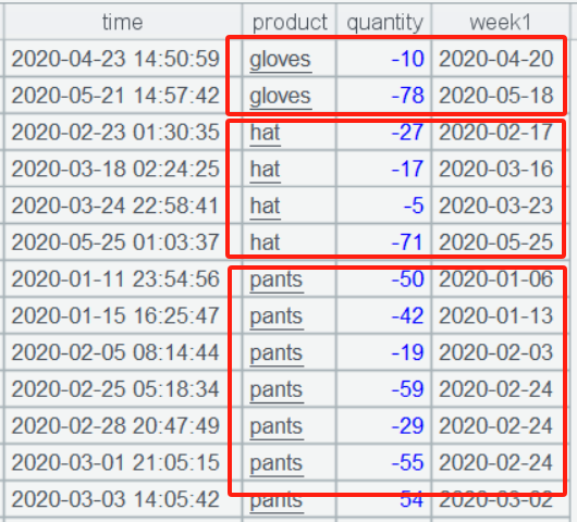
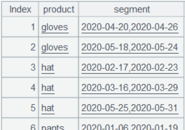
The group() function in A5 uses the @i option to perform conditional grouping. When the condition expression evaluates to true, a new group is created. Here, product[-1] represents the product of the previous record, and week1[-1] represents the Monday date of the previous record. These values are compared with the current record’s product and date to check for continuity. The grouping result is a two-layer nested set:

In A6, the start and end dates of the time period are directly obtained from each consecutive week grouping subset. Here, ~ represents the current grouping subset, ~.m(1) is the first record, ~.m(1).week1 is the first Monday, ~.m(-1) is the last record, and ~.m(-1).week1+6 is the last Monday plus 6, which represents the end of the time period:

3. Calculate the time periods of stock-out weeks and the average weekly sales volume for each product

While accumulating the quantity for the union of purchase and sales records, calculate the Monday date of the week they belong to. Group the data by product and Monday date, then select groups with stock-out occurrences (where cumulative quantity equals 0). Aggregate the total sales volume of these stock-out weeks. Subsequent logic follows the previous problem: group consecutive stock-out weeks, calculate their time periods and the average weekly sales volume (total sales volume of multiple stock-out weeks / number of weeks).

SQL:

with recursive t1 as (
  select time,product,-quantity quantity from sales
  union all
  select * from purchases
),
t2 as (
  select *, sum(quantity) over(partition by product order by time) cum
  from t1
),
t3 as (
  select product, date_sub(date(time), interval weekday(time) day)	week1
  from t2
  where cum=0
  group by 1, 2
),
t4 as (
  select *, row_number() over(partition by product order by week1) rn
  from t3
),
t5 as (
  select product, min(week1) start, min(week1) week1, rn
  from t4 
  group by product
  union all
  select h.product, (case when datediff(h.week1,q.week1)>7 then h.week1 else q.start end), h.week1, h.rn
  from t4 h join t5 q
    on h.product=q.product and h.rn=q.rn+1
),
t6 as (
  select product, start, max(week1)+interval 6 day end
  from t5
  group by product,start
),
t7 as (
  select product
    ,date_sub(date(time), interval weekday(time) day) week1 
    ,sum(quantity) quantity
  from sales
  group by 1,2
)
select t6.product, concat(start,',',end) segment, avg(t7.quantity) avg
from t6 join t7
  on t6.product=t7.product and t7.week1 between t6.start and t6.end
group by 1,2
order by 1,2;

In SQL, each individual (sub)query operation is performed on the entire dataset. It is difficult to define complex or composite operations on grouped subsets during computation. Therefore, calculating the time periods of stock-out weeks and the total sales volume per week must be performed separately on the entire dataset, and the results of these two operations are then associated.

SQL can perform pure grouping, where the resulting grouped subsets still contain detailed data. This makes it convenient to define complex calculations for each group. When writing scripts, you can follow a natural, step-by-step approach without needing to rack your brain for alternative solutions:

	A
1	=file("purchases.txt").import@t()
2	=file("sales.txt").import@t().run(quantity=-quantity)
3	=(A1|A2).sort(product,time).derive(cum(quantity;product):cum,pdate@w1(time):week1)
4	=A3.group(product,week1).select(~.pselect(cum==0))
5	=A4.new(product,week1,-~.sum(if(quantity<0, quantity)):quantity)
6	=A5.group@i(product!=product[-1] || week1-week1[-1]>7)
7	=A6.new(product, week1/","/(~.m(-1).week1+6):segment, ~.avg(quantity):avg)

A3: Union purchase and sales records, sort by quantity, and calculate cumulative quantity (cum) and Monday date (week1).

A4: Group by product and Monday date, and use pselect to identify weeks where stock-outs occurred.

A5: Aggregate the total sales volume for the stock-out weeks.

A6: Group according to condition, placing consecutive stock-out weeks into the same group.

A7: While calculating the start and end dates of the time period, aggregate the average weekly sales volume.

Download test data